This is a second attempt at this posting. The first attempt got 60% of the way done, then I rebooted my machine before I saved the posting… Doh. So let’s try this again:

Every once in a while I feel the need to stop exploring all the new and cool stuff in the world of workbench and do a deep dive into something that involves names which are restricted to eight characters or less. Something that involves a script rather than a GUI click. Something that requires you to look at a real equation, something with an integral sign in it:
I want to learn about something that uses comma-delimited commands.
So, up comes ANSYS Help, dive down into the release notes for Mechanical APDL and look for something obscure but useful. New elements… Aha! HSFLD21 – now that is a name to make any I-only-use-the-GUI-and-manuals-with-equations-but-without-color-animations-make-me-nervous user cringe. Hydrostatic. I like that word. It reads:
This 2-D hydrostatic fluid element models fluids that are fully enclosed by 2-D planar and axisymmetric solids. This element is well suited for modeling fluid-solid interaction with incompressible or compressible fluids under uniform pressure. It can be used in geometrically linear as well as nonlinear static and transient dynamic analyses.
Now I have something I can sink my teeth in.
The Basics on the HSFLD241 and HSFLD242
New at R13, these elements are used to model compressible or incompressible fluids that are surrounded by solids. The key assumption to be aware of is deserving of its own line:
The fluid volume has uniform pressure, temperature, and density without any gradients
So no sloshing, variation due to gravity, etc.. Take a look at FLUID80 if you want these things… maybe a future article topic.
HSFLD241 is the 2D and axisymetric version, and HSFLD242 is the 3D version. If you look at the element pictures from the manual at the top of the posting you’ll see that they are a surface effect element with an extra node, called a pressure node. You use ESURF to apply the element to the inside face of your enclosing volume, and you link all the faces that make up the volume by making them share a node (L or Q). The fact that they all share the same node tells the solver that they make a volume. Besides sharing the node, they must share the same material and real number.
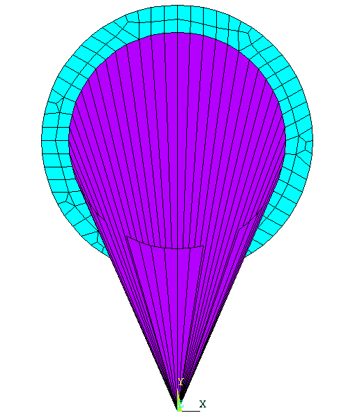
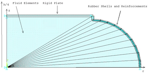
When you use ESURF to make the elements, it automatically makes them a positive volume by the order it defines the face nodes with. But sometimes you may want to create a negative volume inside your positive. Say you are modeling a tire (what this element was added for actually) and you will find that the pressure node is outside of the volume. The calculated volume is not correct. You need to subtract volume for the elements that are actually not in your volume. Here is a cross section to try and make more sense of it.

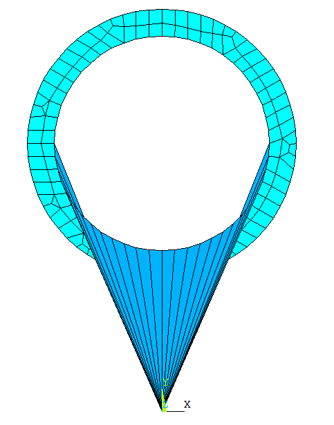
The purple parts are the fluid. So this is not right. You need to go in and create negative elements on any faces that face away from the origin. You do this in two steps: Mesh using ESURF like you normally would, then grab the elements you want to turn into negative elements and issue the ESURF,pnode,REVERSE command. This will turn those elements into negative volumes. The key hear is to create your geometry in a way so that you can easily select faces that point away from the center of your volume. If you don’t, you will need to write a macro that loops through the elements, checks the vector from the face centroid to the center of you volume and if it facing out, swap the element normal. Not hard, just tedious. In our example, the negative element will look like this (color changed for clarity):

DOF’s:
The elements have displacement (UX,UY and UX,UY,UZ) Degrees of Freedom on the face part of the element, the part that sits on your structural elements. The pressure node has a DOF of HDSP or hydrostatic pressure by default, and both PRES and HDSP if you set KEYOPT(1) = 1. This is so you can hook the node to other elements that have PRES DOF’s like the FLUID116.
Real Constants
For real properties you have the ability to specify a thickness (defaults to 1) on the 2D element so the program can calculate volume correctly. Both versions have a real constant of PREF, the reference pressure. Simple enough.
Material Properties
If you opt for an incompressible fluid, just specify a density and coefficient of thermal expansion for your material. But if you are modeling a compressible fluid, you use a new material property table to specify the material properties: TB,FLUID. Within the FLUID model you have three options: a model for liquids, a model for gases, or you can provide pressure-volume data. It is recommended that you read the theory manual on these three to understand the difference and how to use them, as well as the standard command information for the TB.
For TB,FLUID,,,,LIQUID the model is basically a squishy solid. You give a bulk modulus, coefficient of thermal expansion, and an initial density over up to 20 temperatures.
For TB,FLUID,,,,GAS you simply give a Density. The program then simply uses the Ideal Gas Law… you remember that from freshman physics? Or was it chemistry. I kind of remember it… sort of:
If you have a compressible fluid that does not follow the idea gas law, then you can supply your own pressure vs. volume table with TB,FLUID,,,,PVDATA.
KEYOPT
KEYOPT(1) controls the DOF’s on the pressure node. By default the uniform pressure for the solid is stored as HDSP. If you set KEYOPT(1) to 1, then a PRES DOF is added and is set to be equal to HDSP. This is so you can hook a FLUID116 up to it and flow out of your volume… more below.
KEYOPT(3) is used on the HSFLD241 element to say if it is Planer (0) or Axisymmetric (1)
Use KEYOPT(5) to turn on mass effects for the elements. Remember, this is a uniform mass. But if you have gravity or you are doing a modal analysis, you need this turned on.
Turn compressibility off by setting KEYOPT(1) to 1.
Other Basic Info
Give the manual page a read on the element. There are a lot of output options besides the DOF solution. Stuff like Volume, Mass, and mass flow rate.
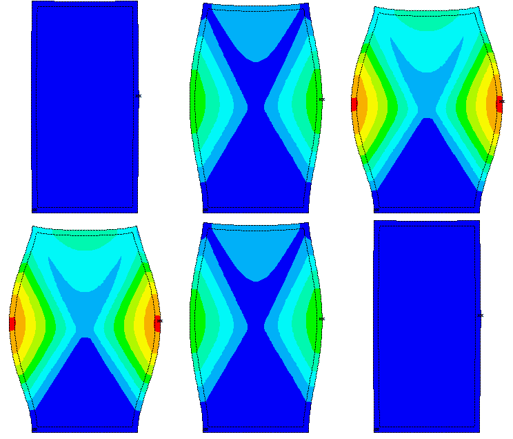
Simple Example
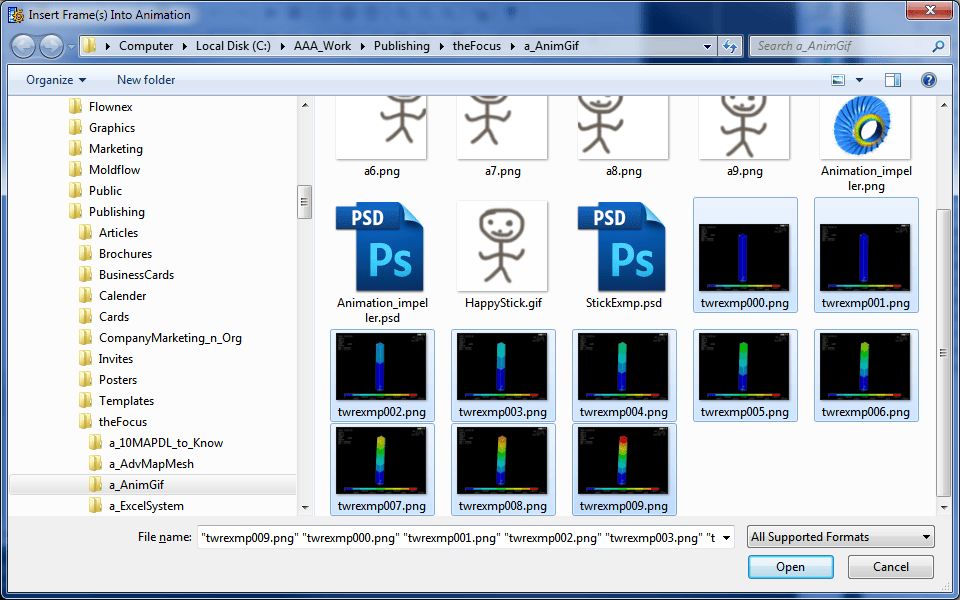
(Want to know how I made this animation… that will be next weeks article.
I used a program called GIF Movie Gear, best $29.95 I’ve spent in a while…)
So, having waded through the boring bits, let’s build a model. Our first example is simply a 2D hollow rectangle that we apply a pressure to. Here is the macro. Take a look at the comments and follow the process.
 !Square Baloon Macro   - Example for HDSP241
 !
 ! Get in the begin level, clear the databse
 !   and go to the preprocessor
 finish
 /clear
 /prep7
 ! Define Dimensions as parameters
 wdth = 2
 hght = 4
 thk = .1
 ! Build two rectangles and subtract the inner one
 !  to make an enclosure
 blc4,(-1*wdth/2),0,wdth,hght
 blc4,(-1*wdth/2)+thk,thk,wdth-2*thk,hght-2*thk
 asba,1,2
 ! Make a component out of the inner lines - this is
 !  where we will put our HDSP elements
 lsel,s,,,5,8
 cm,l_insd,line

 ! Define a 182 for the solid and 241 for the fluid
 et,1,182
 et,2,241

 ! Sort of soft material for the enclosure wall
 mp,ex,1,10e5
 mp,nuxy,1,.3
 mp,dens,1,.001

 ! Some fluid properties
 tb,fluid,2,,,,liquid   ! Liquid Properties
 tbdata,1,300000        ! Bulk Modulous
 tbdata,2,6.4e-4        ! Coeficient of thermal exp.
 tbdata,3,.001          ! Density

 ! Mesh the enclosure wall
 type,1
 mat,1
 esize,thk/2
 amesh,all

 ! Grab the inside nodes from the compenent and create
 !   the fluid mesh using esurf
 cmsel,s,l_insd
 nsll,s,1
 type,2
 mat,2
 n,999,0,2
 esurf,999  ! Tell esurf to make the "extra" node 999
            ! That all the elements share
 allsel,all

 ! Fix the bottom of the enclosure vertically
 !  And fix the bottom right corner tangentially
 !  to constrain the model
 nsel,s,loc,y,0
 d,all,uy
 nsel,r,loc,x,-1*wdth/2
 d,all,ux
 allsel

 ! Specify an load of 100 psi as the internal pressure
 !  The model will ramp up to that load over the specified
 !  substeps
 d,999,hdsp,100

 ! Set up Solve and Run
 /solu
 nlgeom,on
 nsubst,50,100,20
 outres,all,all   ! Don't forget to save substeps so you
                  !   can animate them
 solve
 finish

 ! Animate the resulting displacement
 /post1
 set,last
 /dscale,1,1
 plnsol,u,sum
 andata,0.5,,0,0,0,1,0,1
One key thing to note in the code is the ESURF command. Notice how you specify the common node as the first argument in the command. This is pretty useful and avoids making you go through and specify. You can download the macro here.
A More Complex Example
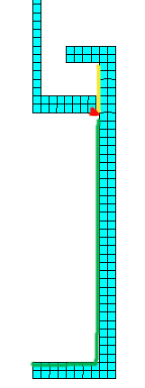
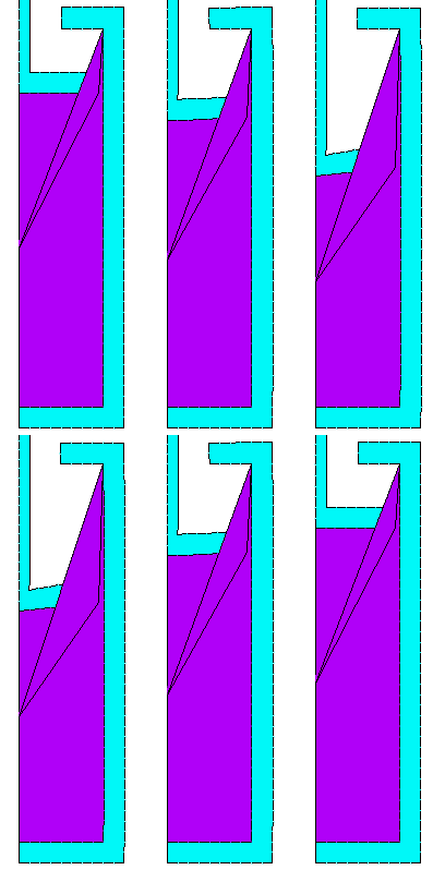
The help on this element is pretty cool, and it even includes an example of how to build a piston. Unfortunately, it does not include the part that solves it. So I’ve added that made some other changes, including an animation and a short trip into POST26 to get pressure and volume of the fluid over time. The code is below. The most obvious thing when looking at this animation is the funny triangle thingy. that is a negative element that deals with the fact that the volume is changing over time. It is not 100% accurate but basically says any fluid above the piston needs to be subtracted. In the image on the right, the solid geometry mesh, you can imagine that your fluid volume can be anywhere inside the piston, from the top of the yellow line to the whole length of the green. The red dot shows the bottom corner of the piston. If you make an element from the red dot to the top and bottom of the yellow line, no mater where the piston goes you will subtract the volume of any part of the total volume that is above the piston. I found that kind of slick and clever of the ANSYS developers. It doesn’t plot so cool, but it gets the job done.
Here is the code:
 finish
 /clear
 /prep7
 ! Define element types
 et,1,182    !plane182
 keyopt,1,3,1    !axisymmetric option
 et,2,241    !hsfld241
 keyopt,2,3,1 ! axi option
 ! Material properties for Steel
 mp,ex,1,2.0e5    !Young's Modulus in N/mm^2
 mp,nuxy,1,0.3    !Poisson's ratio
 mp,dens,1,7.7e-9!Density in ton/mm^3

 ! Material properties for hydraulic fluid
 tb,fluid,2,,,,liquid
 tbdata,1,2000.0    !Bulk Modulus in N/mm^2
 tbdata,2,6.4e-4    !Coefficient of thermal expansion
 tbdata,3,8.42e-5!Density in ton/mm^3
 ! Nodes
 n,1,0.0,50.0    !pressure node
 ! Keypoints
 k, 1, 0.0,  0.0
 k, 2,25.0,  0.0
 k, 3,25.0,100.0
 k, 4,10.0,100.0
 k, 5,10.0, 95.0
 k, 6,20.0, 95.0
 k, 7,20.0,  5.0
 k, 8, 0.0,  5.0
 k, 9, 0.0, 80.0
 k,10,19.0, 80.0
 k,11,19.0, 85.0
 k,12, 3.5, 85.0
 k,13, 3.5,185.0
 k,14, 0.0,185.0
 ! Areas
 a,1,2,3,4,5,6,7,8
 a,9,10,11,12,13,14
 ! Planar elements
 type,1
 mat,1
 esize,2.5
 amesh,all
 ! Hydrostatic fluid elements--automatic generation
 type,2
 mat,2
 lsel,s,line,,6,9
 nsll,s,1
 esurf,1
 allsel,all
 ! Create the Negative volume element- needed to take into account
 ! the movement of the piston
 e,61,162,,1    !element with negative volume--nodes 61 and 162 swapped
 ! Symmetry boundary condition on pressure node   [REQUIRED]
 d,1,ux,0.0
 ! Symmetry boundary condition on planar mesh
 lsel,s,line,,8,14,6
 nsll,s,1
 d,all,ux,0.0
 allsel,all
 ! Fixed boundary condition on planar mesh
 lsel,s,line,,1
 nsll,s,1
 d,all,all,0.0
 allsel,all

 ! Grab the nodes on top and apply a downward displacement
 nsel,s,,,179
 nsel,a,,,219
 cm,ptop,node
 d,ptop,uy,-35

 ! Run the model
 finish
 /solu
 nlgeom,on
 nsubst,200,500,10
 outres,all,all
 solve

 ! Go to post 26 and get pressure and volume over time
 /post26
 numvar,200
 ESOL,2,180,1 ,NMISC,2,NMISC2_2
 nsol,3,1,HDSP
 /grtyp,2
 plvar,2 ,3

 !Animate the results
 /post1
 set,last
 /dscale,1,1
 /pnum,mat,1
 /number,1
 /edge,1,1
 !esel,u,,,eflp
 pldisp
 andata,0.1,,0,0,0,1,0,1
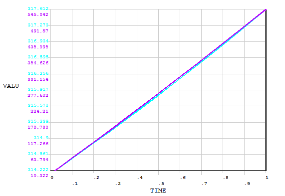
Here is the graph of the results. Not very exciting.
Download the Macro here:
Other things to know
OK, this was a lot more involved than planned, and there is still more to learn. But I’ve got HR paperwork to fill out so we will wrap it up.
You should go through the verification problem for this element: VM209
- You can connect different volumes with FLUID116 elements. This allows some pretty fancy system modeling. Add in some control elements and electromagnetics and you can really capture some complex systems.
- Be very aware of the negative volume issues when modeling tires and such.
- After I started on this article I found out that we are in the middle of a project for a customer who is modeling an optical device that has a fluid core. It is working very well for them. I wish I could show the model, but I would be shot by the customer. I can say that we are getting much better results than when we modeled the volume with solids.
- The FLUID80 is a solid fluid volume element that does take into account non-uniform pressure, mass, etc… Take a look at it if these guys don’t do what you need.
- Can you do this in Workbench? Sort of. You should be able to write a macro that uses a component to create your hydrostatic elements and define the material properties. You won’t be able to post process the results but you can at least set it up and bring back plots. (check out this presentation, slide 41)


