Unable to converge. Convergence Failure. Failure to Converge. Never nice words to see when you are trying to get your simulation done.
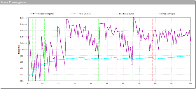
If you’ve encountered convergence failures while running nonlinear structural analyses in ANSYS Workbench Mechanical, this two part series is for you. What is a convergence failure? In a nutshell it means that there is too much imbalance in the system. The calculated reaction forces do not match the applied loads and even though the program tries hard to make changes to overcome the imbalances, it hasn’t been able to do so and stops. If we look at the Force residuals under Solution Information, we will see that the solver has been unable to get the force convergence residual, or imbalance force, to drop below the current criterion
Test model example: Newton Raphson Convergence Failure; Solution Stops
We won’t spend a lot of time here explaining the Newton-Raphson method, convergence, and residual plots here, since we wrote a Focus article back in 2002 which discusses them in more detail. The article begins on p. 7 at this link:
/wp-content/uploads/oldblog/archive/PADT_TheFocus_08.pdf
The context of that article was Mechanical APDL, but the article is directly relevant since solving in Workbench Mechanical is done in Mechanical APDL in batch mode.
In crayon terms, we want the purple line to drop below the blue line. When it doesn’t and the solver is out of options to keep trying, the solution stops and we get an error message.
Now what? The traditional knobs to turn are to increase the number of substeps, decrease contact stiffness if contact is involved, perhaps add more points to the plasticity curve, etc. But what if something else is the problem? How can we identify where the problem is?
In this part I article we will discuss how to plot the Newton-Raphson residuals as contour plots to see where in the model the highest force imbalances are located. Often this is useful information to help us figure out what is going on so we can take corrective action. First, be aware that we must turn on the Newton-Raphson residual plots prior to solving. That means you either have to turn them on and re-solve after a convergence failure, knowing that you’ll get the same failure again, or you need to clairvoyantly (or perhaps just prudently) turn on the residuals prior to attempting the initial solve. Why aren’t they on all the time, you ask? Most likely because they slow things down just a bit and also require a bit more disk space than otherwise, although if the solution runs to completion no Newton-Raphson residual plots are saved.
Here is how we turn them on. In the Details view for the Solution Information branch, change the Newton-Raphson Residuals setting from the default of zero to a nonzero number such as 3 or 4. That will continuously save the last 3 or 4 Newton-Raphson residual plots for viewing as contour plots after the solution has stopped due to a convergence failure.
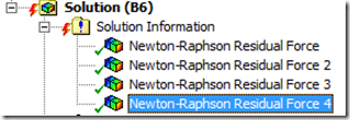
After the solution has stopped, the Newton-Raphson residual plots will be available under the Solution Information branch.
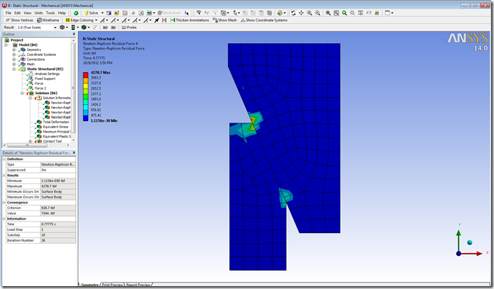
The quantity plotted is actually the square root of the sum of the squares of the residuals in the global X, Y, and Z directions. So, the plots don’t show us direction information, but they do show where the residuals and hence the force imbalances are the largest. Below is an example. The region in red shows where the residuals are the highest. Since this is a model involving contact between two bodies, apparently the contact regions and specifically contact at the corners of the part on the left is the source of our convergence difficulties.
Newton-Raphson Residual Force Plot for the last attempted equilibrium iteration.
So, how do we use this information? In this case we now suspect that the contact regions, especially at the corners of the smaller part, are the problematic areas. Using this information we made two changes to the model.
First, we changed the Detection Method for the contact elements from Program Controlled (at the element Gauss points) to Nodal-Normal to Target. Many times when contact problems involve touching at corners, the robustness of the contact interface can be improved by changing the detection method from Gauss points to nodes.
Second, we reduced the contact stiffness by changing Normal Stiffness from Program Controlled (factor of 1.0) to a Manual setting of 0.2. Reducing the contact stiffness can help with contact convergence for a lot of problems. Too low of a stiffness value can cause problems too, but in this case the resulting penetration is still small so a value of 0.2 seems reasonable. When in doubt, a sensitivity study can be performed whereby you make changes to the contact stiffness value while tracking your results quantities of interest. As with most inputs you can vary, your results of interest should not be sensitive to contact stiffness.
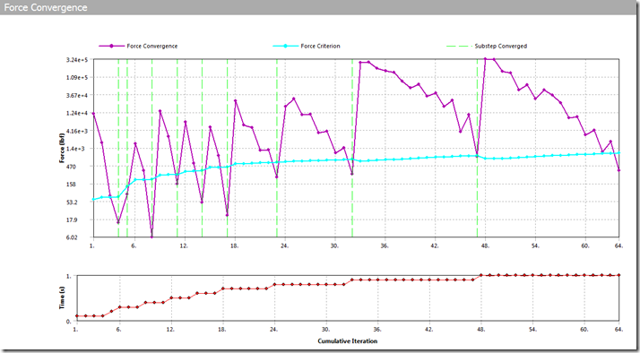
These two changes allowed our test model to nicely converge for the full amount of load.
Other considerations:
The Newton-Raphson Residual plots are always displayed on the original geometry, not the deflected geometry at version 14.0 of ANSYS Mechanical. If the deflections are large this can make it harder to ascertain what is causing the high residual values. In those cases, it can be helpful to compare the total deformation and stress plots for the unconverged solution, along with those plots for the last converged solution, with the 1.0 true scale on the deformation active. This will show the parts in their deflected state, and that can help in determining why the residuals are high at certain locations.
We recommend creating at least 3 residual plots (set in the details of Solution Information as described above). Sometimes the location of the imbalance can bounce around a bit from equilibrium iteration to equilibrium iteration, so having more than one or two plots to look at can be beneficial in determining problem locations.
Conclusion
Summing it up, the Newton-Raphson residual plots are one piece of information we can use to determine why we are having convergence difficulties. They can give us an indication of where the convergence difficulties are occurring in the model, and many times we can use that information to help us know what settings should be modified or what other changes should be made to the model to improve the convergence behavior.
In part II of this article, we’ll look at how to quickly use ANSYS Mechanical APDL to view the elements that have undergone too much deformation.


