 What is the software tool that we numerical simulation types use almost as much as ANSYS products, maybe even more? Most of you will answer Microsoft Excel. We all use it almost every day for a variety of things. Every time I see someone doing something sophisticated with Excel, I learn something new, a tool I can use to be more efficient.
For this week’s The Focus posting, I will be sharing some stuff in Excel, tips, and tricks, that ANSYS users should find useful. I am using Microsoft Excel 2010, and the assumption is that the reader is a good user of Excel, maybe not an expert, but good. I have tried to pick things that have a direct impact on user efficiency. You may already know some or even most of these things, but hopefully, you will find some of it useful. If you have something to share, please add it to the comments.
Take the Time to Setup Tables
I love tables. I’m always getting made fun of because I always convert what I’m working on into tables. Why are they so great?
- They auto-format
- They have filtering built in
- You can refer to the table, columns, rows, and cells in equations with names rather than ranges
- When you add a formula in a column, it automatically copies it to the whole table (my favorite)
- It does automatic totals, averages, etc…
Making a table is easy:
- Select the columns you want in your table
- It is a good idea to have the headers defined
- Go to the Insert Tab
- Click on Table
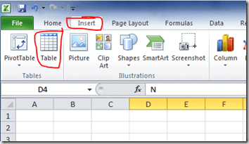
That give you:
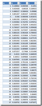
Click on the downward-facing triangle icons to filter. Use the options in the Table Tools > Design tab to set the name, remove duplicates, turn on the total row, and change the basic formatting (color). Once you have played with these for a while, you will find you can not live without them, and people will ask you why you use tables so often.
Concatenation
One of the ways that we use Excel is to convert some sort of text data in row/column form into a command, mostly MAPDL commands. A key to this is the ability to concatenate text strings and the values of cells. I’ve even seen someone write a NASTRAN to ANSYS translator in Excel.
To do so you create a formula (start with =) and string together the text you want with ampersands: &
As an example, if we want to add a column to the table we used above to create N commands, we simply click on any of the cells in the empty column next to our table and enter:
=”n, “&[@N]&”, “&[@X]&”, “&[@[Y ]]&”, “&[@Z]
Because we are using a table, the command uses the column reference [@name] from the tables rather than cells. In a non table the command would look like:
=”n, “&$A6&”, “&$B6&”, “&$C6&”, “&$D6
Either way, you are stringing the values in your cells together with text to make a command:
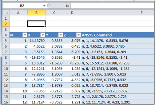
That column can be pasted into a text file, an ANSYS Mechanical code snippet window, or saved to a file.
Text to Columns
After tables, the next most useful feature in Excel for the analyst is the ability to convert the text in a column into multiple columns. This is a lot like the text import window that opens up when you open a text file, but it can be used at any time on any column in your spreadsheet. To use it, simply select the column you want to convert:
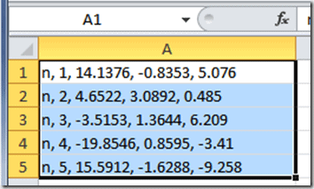
Then go to the Data tab and click on “Text to Columns”

This will bring up the wizard that steps you through the process:
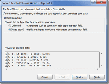
If you are working with a NASTRAN type input file, formatted with fixed columns, you can chose “Fixed Width” here. If not, choose delimited. Click next.
For fixed, you get a ruler that you can drag the column lines back and forth on till you get what you want. Pretty simple.
For delimited, you get the delimiter screen. Specify your delimiter here. In the example, we will use a comma. But it can be spaces, tabs, or any other character. When you specify the delimiter, it shows you how Excel will break it up.
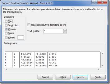
I usually click finish here because the next screen is formatting and I usually play with that once I have the data in Excel.
That is it. Very simple.
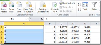
One thing to note, it converts to columns by overwriting columns to the right. So if you have data in those columns, you should insert enough blank columns before you use this command, so you don’t overwrite anything.
Names
Usually you refer to a cell or a range of cells with the old LetterNumber syntax: A3, B7:NN2145, etc… That can be a real pain to deal with and it really doesn’t tell you what the data in that range is. A better way to deal with chunks of information, or critical cells, is to use names.
Creating names is very easy. The simplest is to click on the cell or cells you want to name and then type in the name you want in the input box in the upper left corner:
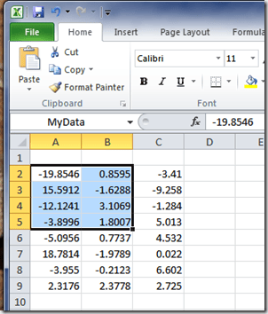
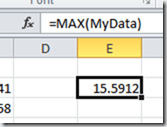
Now, if you want to know the max value of those numbers, you can use the formula =max(MyData)
If I have a lot of constants I want to define, I can use the “Create from Selection” tool in the Formulas tab:
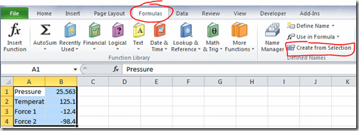
This command brings up a dialog box and you can tell Excel where to grab your names from. Three or Four clicks and you have named parameters instead of cell locations. This is very useful if you have a group of key parameters you want to use in your calculations. Now when you look at your formulas, the descriptive name of the parameters are there rather than a reference.
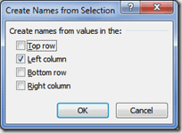
Use the Name Manager in the same Formulas tab to view, edit, and delete your names.
Dynamic Range
A related trick for Excel is creating dynamic ranges. What do you do when you name a range and then the amount of data in that range changes? You have to redefine your range. Nope, you don’t. You can define the range using a formula that changes as the length of the column, or row, changes.
The name can be defined for a column as: =OFFSET(startCell,0,0,COUNTA(column)-1)
Or for a row: =OFFSET(startCell,0,0,0,COUNTA(row)-1)
This may be the most time saving trick I know in Excel.
You put the formula into the “Define Name” dialog box found on the Formulas tab:
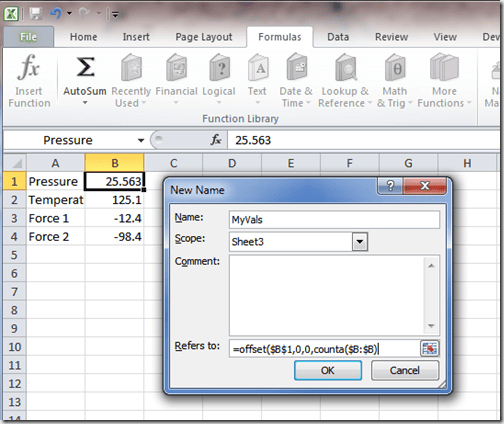
Now, no matter how long the column of data is, MyVals will always contain it. A big time saver.
Relative Reference on Record Macro
How many times have you gotten data in Excel, or imported data into Excel, where you want to make a small change to every line. But you have several thousand lines. If you do a “Record Macro” that doesn’t work because you have to click down to the next line, then run the macro and repeat that over and over again. Wouldn’t it be great if you could simply record a macro with some sort of relative reference.
For years (maybe decades) I didn’t know you could do that. There is an option under the Developer Tab called “Relative Reference.” Click that before you record your macro and you are good to go.

As an example, take a look at this data. Nodal coordinates on one line, rotations on the second.
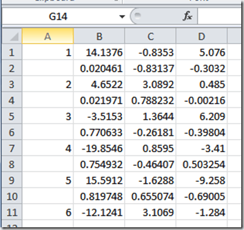
I want to grab the rotations, paste them on the same line as the coordinates, delete the rotation line, then move to the next node.
Here is a video that shows the process:
That is all fine and dandy if you have a few dozen lines, but your fingers will get tired CTRL-e’ing that many times. I quick fix is to go into the macro and add a simple loop. First we use CountA() to see how many nodes we have, then we loop on that with a for statement:
Sub Macro3()
'
' Macro3 Macro
'
' Keyboard Shortcut: Ctrl+e
'
cnt = Application.CountA(Range("a:a"))
For i = 1 To cnt
ActiveCell.Offset(1, 1).Range("A1:C1").Select
Selection.Cut
ActiveCell.Offset(-1, 3).Range("A1").Select
ActiveSheet.Paste
ActiveCell.Offset(1, 0).Rows("1:1").EntireRow.Select
Selection.Delete Shift:=xlUp
ActiveCell.Select
Next i
End Sub
Of course you could have done this with *VREAD’s in MAPDL, or python. But sometimes Excel is just faster.


