
We recently had a tech support request from a customer, asking for the ability to define a spatially varying thermal contact conductance (TCC) on a contact region in ANSYS Mechanical. We came up with a solution for ANSYS 14.5 via an example which includes a couple of verification plots.
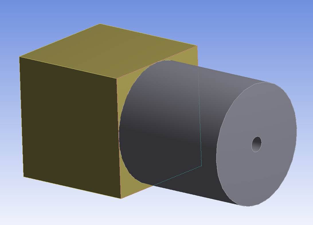
The test model consists of two solids, connected via a contact region. The thermal contact conductance at the contact region was defined as a table, with the rows and columns of the table corresponding to local coordinates within the plane of the contact surface. The table was defined and implemented using Mechanical APDL commands in the Mechanical tree.

Low values of TCC were used for testing purposes. This helped verify that the tabular values were actually being used as intended. A constant temperature was applied to the face at one end of the model, while a different constant temperature was applied to the face at the extreme other end of the model. This temperature differential caused heat to flow through the contact region, subject to the resistance defined via TCC values.
The coordinates in the plane of the contact surface were Y and Z. Thus, the table of TCC values varied in the Y and Z directions, as shown here:
Z
Y | 0.0 1.0
0.0 | 0.0001 0.0005
1.0 | 0.0005 0.0002
Three ANSYS Mechanical APDL command objects were inserted into the tree in the Mechanical editor. The first command object simply added a scalar parameter to keep track of the contact element type/real constant set number for use later:

The second command object was placed in the analysis type branch, meaning this set of commands would be executed just prior to the Solve command. This command object does three things:
1. Defines the TCC table vs. Y and Z coordinates.
2. Reads the table in as an MAPDL real constant for the contact elements identified in the first command object.
3. Issues the command, “rstsuppress,none”. More on this later.
This is how the second command object was defined:

That third step mentioned above was a key to getting this technique to work in 14.5. The rstsuppress command is not documented currently, but Al Hanq of ANSYS, Inc. has told me that it will be documented in the future. The default setting turns off contact results from being written to the results file in a thermal analysis. The idea is to help keep results file sizes from getting excessively large, especially for transient thermal runs. In this case, we actually wanted the thermal contact results in the results file, so we issued “rstsuppress,none” so the thermal contact results were not suppressed.
The final command object was for verification of the applied TCC values. This set of commands generates two plots using MAPDL postprocessing commands. The first plot is of heat flux going through the contact elements. The second plot displays the TCC values for node ‘i’ of each contact element (averaged).
Here is the third command object:

Both of these plots show up in the tree, labeled as Post Output and Post Output 2 in the image above.
This is the resulting thermal flux at the contact surface:

Here is the applied thermal contact conductance, as mapped from the table defined in the second command object:

In summary, we took advantage of Mechanical APDL command objects to apply thermal contact conductance values that vary along the contact region. We also used MAPDL commands to create two plots that help verify that the TCC values were applied as intended. Hopefully this is a helpful example.


