Guest Blogger
We are pleased to publish this very useful post from Nicolas Jobert from Synchrotron SOLEIL in France. Nicolas is a Mechanical Engineer with more than 20 years of experience using ANSYS for engineering design and analysis in academia and industry. He currently is Senior Mechanical Engineer at Synchrotron SOLEIL, the French synchrotron radiation facility. He also teaches various courses on Design and Validation in the field of structural and optomechanics. He graduated from the Ecole Centrale Marseille, France, and is a EUSPEN member.
As Time Goes By
Do you remember the moment you first heard about ANSYS introducing APDL Math?
I, for one, do, and I have a vivid memory of thinking “Wow, that can be a powerful tool, I’m dead sure it won’t be long before an opportunity arises and I’ll start developing pretty useful procedures and tools”. Well, that was half a decade ago, and to my great shame, nothing quite like that has happened so far. Reasons for this are obvious and probably the same for most of us: lack of time and energy to learn yet another set of commands, fear of the ever present risk of developing procedures that are eventually rejected as nonstandard use of the software and therefore error-prone (those of you working under quality assurance, raise your hand!), anxiety of working directly under the hood on real projects with little means to double check your results, to name a few.
That said, finally an opportunity presented itself, and before I knew it, I was up and running with APDL Math. The objective of this article is to showcase some simple yet insightful applications and hopefully remove the prevention one can have regarding using these additional capabilities.
For the sake of demonstration, I will begin with a somewhat uncommon analysis tool that should nevertheless ring a bell for most of you, that is: modal analysis (and yes, the pun is intended). You may wonder what is the purpose of using APDL Math to perform a task that is a standard ANSYS capability since say revision 2.0, 40 years ago? But wait, did I mention that by modal analysis, I mean thermal modal Analysis?
Thermal Modal Analysis at a Glance
Although scarcely used, thermal modal analysis is both an analysis and a design validation tool, mostly used in the field of precision engineering and or optomechanics. Specifically, it can serve a number of purposes such as:
Q: Will my system settle fast enough to fulfill design requirements?
A: Compute the system Thermal Time Constants
Q: Where should I place sensors to get information rich / robust measurements?
A: Compute Thermal modes and place your sensors away for large thermal gradients
Q: Can I develop a reduced model to solve large transient thermal mechanical problems?
A: Modal basis allows for the construction of such reduced problem effectively converting a high-order coupled system to a low order, uncoupled set of equations.
Q: How to develop a reduced order state-space matrices representation of my thermal system (equivalent to SPMWRITE command)?
A: Modal analysis provides every result needed to build those matrices directly within ANSYS.
Although you might only be vaguely familiar with many or all of those topics, the idea behind this article is really to show that APDL Math does exactly what you need it to do: allow the user to efficiently address specific needs, with a minimal amount of additional work. Minimal? Let’s see what it looks like in reality, and you will soon enough be in a position to make your own opinion on the matter.
Thermal Modal Analysis using APDL Math
To begin with, it is worth underlining the similarities and differences between structural (vibration) modes and thermal modes.
Mathematically, both look very much the same, i.e. modes are solutions of the dynamics equation in the absence of forcing (external) term:
|
Domain |
Equation solved |
Terms Explained |
| Structural |
[K] is the stiffness matrix |
|
|
Thermal |
|
[K] is the conductivity matrix |
Now, the fundamental difference is that the eigenvalues have completely different physical interpretations (This is a direct consequence of the fact that dynamical systems are 2nd order systems, whereas thermal systems a 1st order systems. While after being disturbed the former will oscillate around equilibrium position, the latter will return to its initial state via exponential decay. Mind you, there is no such thing as thermal resonances!) :
- Structural : λ=ω², i.e. the square of a circular frequency
- Thermal: λ=1/τ, i.e. the inverse of time constant
No big deal, right? Hence, the APDL Math code for Thermal Modal Analysis should be a straightforward adaption of the original. As it turns out, the modifications are quite small. Below is a table comparing input codes to perform both type of analyses, using APDL Math.

|
Structural |
Thermal |
! Setup Model … ! Make ONE dummy transient solve ! to write stiffness and mass ! matrices to .FULL file /SOLU ANTYPE,TRANSIENT TIME,1 WRFULL,1 SOLVE ! Get Stiffness and Mass *SMAT,MatK,D,IMPORT,FULL,,STIFF *SMAT,MatM,D,IMPORT,FULL,,MASS ! Eigenvalue Extraction Antype,MODAL modopt,Lanb,NRM,0,Fmax *EIGEN,MatK,MatM,,EiV,MatPhi ! No need to convert eigenvalues ! to frequencies, ANSYS does ! it automatically ! Done ! |
! Setup Model
 …

! Make TWO dummy transient solve
! to separately write conductivity
! and capacitances matrices to .FULL file
 /SOLU
 ANTYPE,TRANSIENT
 TIME,1
 NSUB,1,1,1
 TINTP,,,,1
 WRFULL,1

! Zero out capacitance terms
 …
 SOLVE
 ! Get Conductivity Matrice
 *SMAT,MatK,D,IMPORT,FULL, Jobname.full,STIFF
 ! Restore capacitance and zero out
 ! conductivity terms
  …
 SOLVE
 ! Get Capacitance Matrice
 *SMAT,MatC,D,IMPORT,FULL,,STIFF

! Eigenvalue Extraction
 Antype,MODAL
 modopt,Lanb,NRM,,0,1/(2*PI*SQRT(Tmin))
 *EIGEN,MatK,MatC,,EiV,MatPhi

! Convert Eigenvalues for Frequency
! to Thermal time Constants
!
 *do,i,1,EiV_rowDim
    Eiv(i)=1/(2*PI*Eiv(i))**2
 *enddo

! Done !
|
The only data requested from the users is the number of requested modes (NRM) as well as the upper frequency (or for that matter, the shortest time constant of interest). Also, note that in the thermal case, one needs to perform two separate dummy analyses to store the conductivity and capacitance matrices, since internally those are merged into an equivalent stiffness (conductivity) matrix:

If you are familiar with APDL, some important differences are apparent here:
- Results from the eigenvalues are stored in a vector (EiV) and a matrix (MatPhi), which need not be declared but are created when executing the *EIGEN command (no *DIM required).
- For each APDL Math entity, ANSYS automatically maintains variables named Param_rowDim and Param_colDim, hence removing the burden to keep track of dimensions.
But where on Earth is my eye candy?
Now that we have some procedure and results, we would like to be able to show this to the outside world (and to be honest, some graphical results would also help getting confidence in results).
The additional task to do so is really minimal. What we need to do is simply to put back those numerical results into the ANSYS database so that we can use all the conventional post-processing capabilities. This can be made using the appropriate POST1 commands, essentially: DNSOL. And, while we are at it, why not do a hardcopy to an image file? Here is the corresponding input.
 … User should place all nodes with non-prescribed temperatures in a component named MyNodeComponent

… First, convert Eigenvectors from solver to BCS ordering
 ! Conversion needed
 *SMAT,Nod2Bcs,D,IMPORT,FULL,Jobname.full,NOD2BCS
 *MULT,Nod2Bcs,TRAN,MatPhi,,MatPhi

! Then, read in mapping vector to convert to user ordering
 *VEC,MapForward,I,IMPORT,FULL,Jobname.full,FORWARD

! Put the results in ANSYS database
 /POST1
 *do,ind_mode,1,NRM
 cmsel,s,MyNodeComponent
 curr_node=0
 *do,i,1,ndinqr(0,13)
 curr_node=ndnext(curr_node)
 curr_temp=MatPhi(MapForward(curr_node),ind_mode)
 dnsol,curr_node,TEMP,,curr_temp
 *enddo
 Tau=1/(2*3.14*EiV(ind_mode))**2

To=NINT(Tau*10)/10 ! compress to 1 digit after comma
 /title,Mode #%ind_mode% - Tau=%To%s
 plnsol,temp
 ! Hardcopy to BMP file
 /image,SAVE,JobName_Mode%ind_mode%,bmp
 *enddo
This way, modes can be displayed, or even written to a conventional .RTH file (using RAPPND), and used as any regular ANSYS solver result.
Nice, but an actual example wouldn’t hurt, would it?
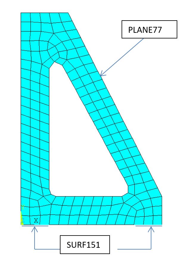
Now you may wonder what the results look like in reality. To remain within the field of precision engineering, let’s use a support structure typically designed for high-stability positioning. From a structural point of view, it must have a high dynamic stiffness and a low total mass so that a Delta shaped bracket is appropriate. Since we want the system to rapidly evacuate any heat load, we choose aluminum as candidate material. We do know from first principles that any applied disturbance will exponentially vanish and the system will go back to equilibrium state. Now, what will be the time constants of this decay?
For the sake of simplicity we restrict the analysis to a highly simplified, 2D model of such a support. PLANE55 elements are used to model the structural part while the heat sink is accounted for using SURF151. Boundary conditions are enforced using an extra node.
After applying boundary conditions, we execute the modal solution to obtain say – the first 8 modes.
| Index | Time Constant [s] | Comment |
| 1 | 535.9 | Quasi-uniform temperature field (i.e. “rigid body” mode) |
| 2 | 32.1 | 1st order (one wavelength along perimeter) |
| 3 | 23.8 | 1st order (one wavelength along perimeter) |
| 4 | 8.1 | 2nd order (two wavelengths along perimeter) |
| 5 | 6.8 | 2nd order (two wavelengths along perimeter) |
| 6 | 3.5 | 3rd order (three wavelengths along perimeter) |
| 7 | 3.1 | 3rd order (three wavelengths along perimeter) |
| 8 | 2.2 | 4th order (four wavelengths along perimeter) |
The output is strictly the same as the one a standard modal analysis, except for the two additional lines at the end of the solving sequence.
Allocate a [8] Vector : EIV

Allocate a [227][8] Dense Matrix : MatPhi
Please note that the solution has 227 DOFs whereas the entire problem has 228 DOFs. This is the consequence of having introduced the boundary conditions as an enforced temperature on a node, which DOF is therefore removed from the DOF set to be obtained by the solver.
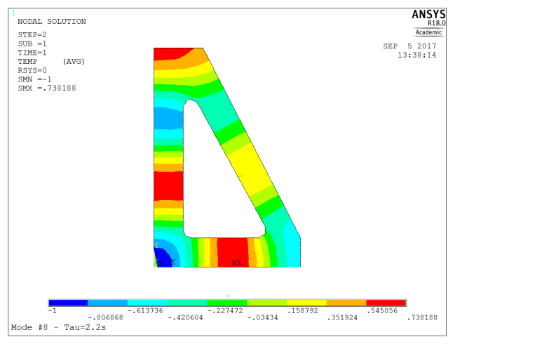
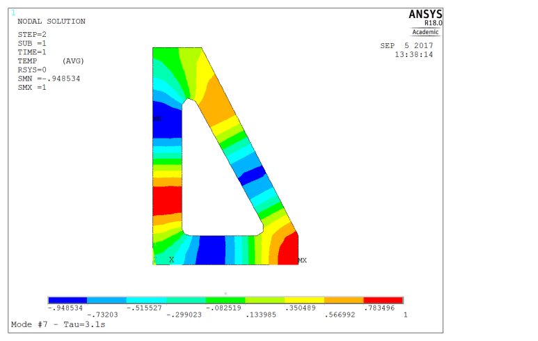
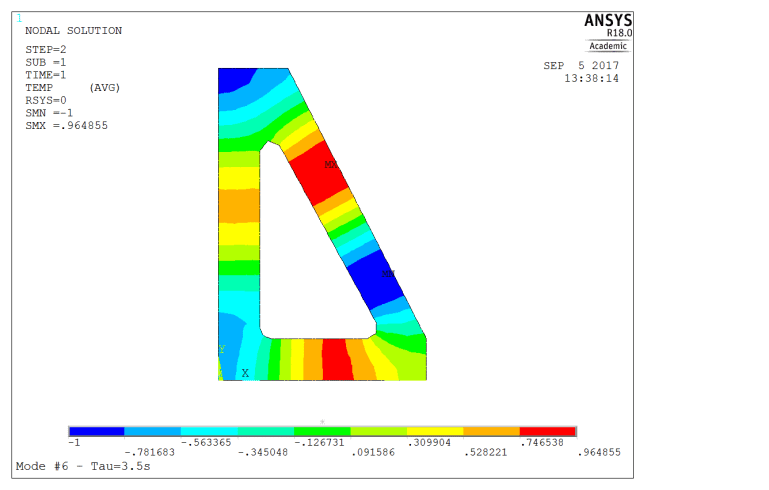
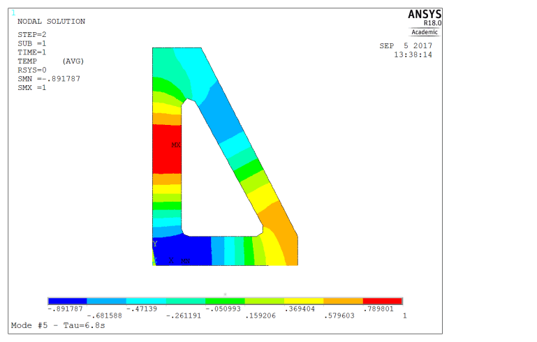
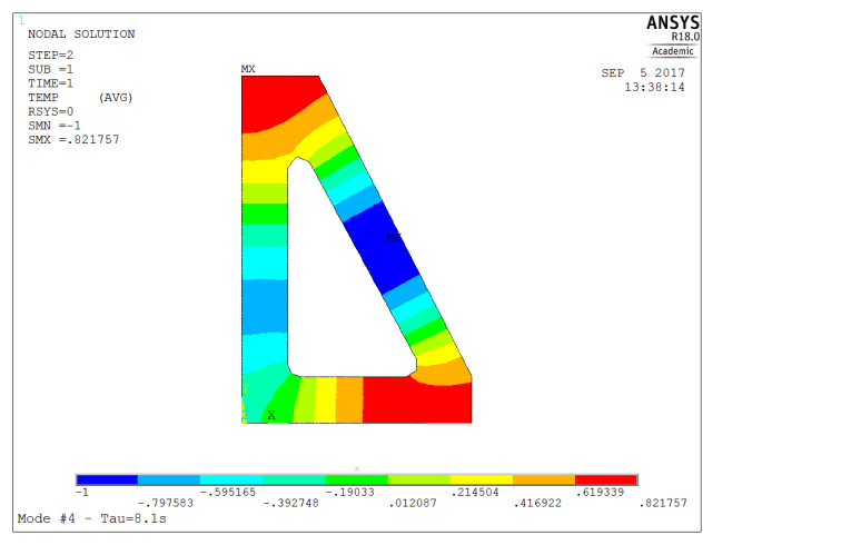
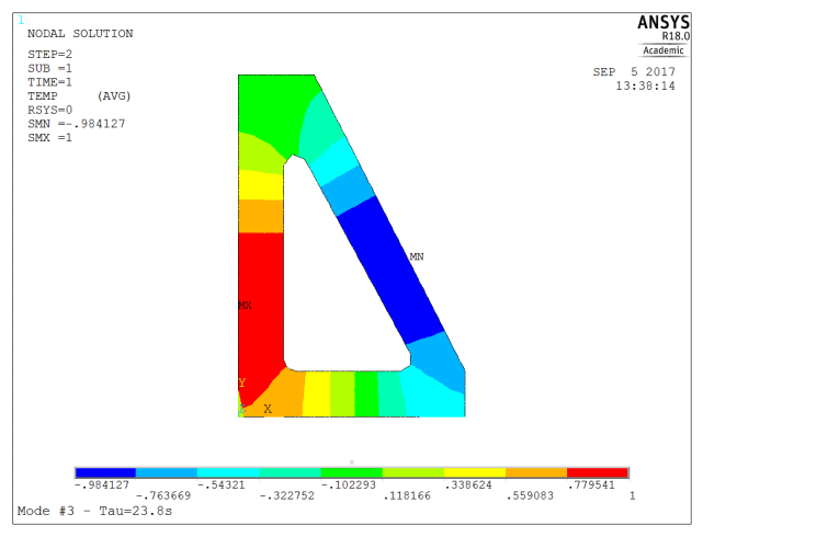
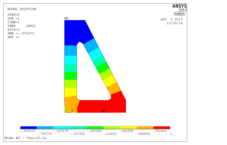
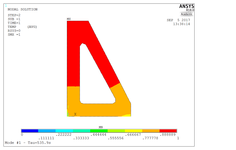
Also, we might want to use the modal shapes information to decide which locations are best suited to capture the entire temperature field on the structure. Without knowledge of the excitation source, one straightforward way to do so is to retain for each mode the node that has the largest amplitude. This is made even easier in this situation, since we have normalized each mode to have unit maximum amplitude we just need to select nodes having modal amplitude equal to 1 (or -1). On the figure below, each temperature sensor location is marked with a ‘TSm’ label where m is the mode index.
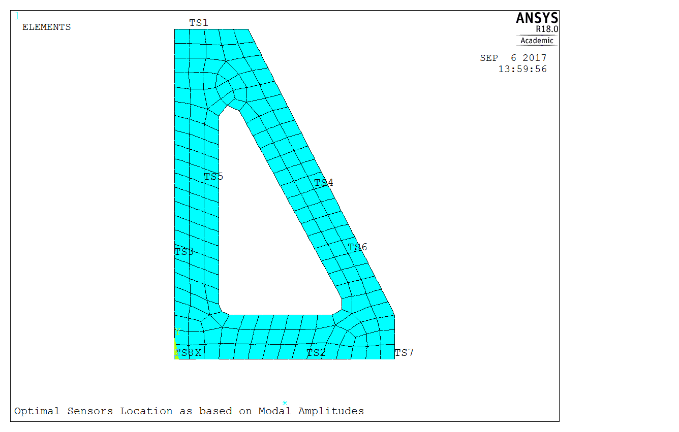
Doing so, we reach a pretty satisfactory distribution for the sensors locations, completely consistent with intuition. In numerical terms, we can also check that the modal matrix [Φ]_sensors, i.e. the original full matrix restricted to the selected DOF, has an excellent condition number. But there are many other things we could do starting from this. For example, with additional information, such as the location and the frequency content of the temperature fluctuations, one could further restrict the set of needed temperature sensors by running a dummy transient analysis and choosing locations where the correlation between sensors readings is as low as possible (using *MOPER,,,CORR). Even better, one can estimate the thermally induced displacements and select locations best suited to build an empirical model (typically using AR or ARMA), allowing one to predict structural displacements induced by temperature fluctuations using just a couple of sensors. This in turn can be used to select control strategies, check modal controllability… all within ANSYS.
Conclusion
APDL Math was presented as an alternate route for users who need to include specialized steps in an otherwise standard FE process, and in my opinion it does just that. The benefits can be immense and the learning curve is steep but short. As long as the user knows what he/she is doing, there is little possibility to get lost: after all, APDL Math only comprises 18 additional commands.
What hindered me so far was the necessity to account for internal, BCS and user ordering, but it really is not a big deal, as seen from the above example.
What is more, the possibility to store the created results in the Mechanical APDL database (DNSOL and RAPPND are your friends!) provides every means to control your results and finally to build confidence in your developments.
And for those of us who prefer to stay within Workbench environment, there is nothing preventing from including APDL Math procedures into Workbench command snippets.
This was just an introductory example, since many other applications could be found, to name a few just in the fields of precision engineering and/or opto-mechanics:
- Speed up transient thermal mechanical analyses
- Perform harmonic analysis of thermal models
- Virtual testing of physical setup, including real-time control systems (model based)
- Modal testing, error localization, automated model updating
Let us know your opinion on the matter, and if further introductory articles on APDL Math could be of use to the ANSYS users community.


