One of the problems we can encounter in a nonlinear structural analysis in ANSYS Mechanical is that elements become so distorted that the solver cannot continue. We get messages saying the solver was unable to complete, and the solver output will contain a message like this one:
*** ERROR ***                           CP =      37.969   TIME= 14:40:06
  Element 2988 (type = 1, SOLID187) (and maybe other elements) has become
  highly distorted.  Excessive distortion of elements is usually a
  symptom indicating the need for corrective action elsewhere.  Try
  incrementing the load more slowly (increase the number of substeps or
  decrease the time step size).  You may need to improve your mesh to
  obtain elements with better aspect ratios.  Also consider the behavior
  of materials, contact pairs, and/or constraint equations.  Please rule
  out other root causes of this failure before attempting rezoning or
  nonlinear adaptive solutions.  If this message appears in the first
  iteration of first substep, be sure to perform element shape checking.
The Solution branch will have the telltale red lightning bolts, indicating the solution was not able to complete due to nonconvergence.

If you are not aware, one technique we can use to get past this problem of excessive element distortion is to have ANSYS automatically remesh the model or a portion of the model while the solution is progressing. The current state of the model is then mapped onto the new mesh, in the currently deflected state. In this manner we can automatically continue with the solution after a slight pause for this remeshing to occur. Minimally all we need to do as users is insert a Nonlinear Adaptive Region under the Static Structural branch, and review and specify a few settings (more on this later).
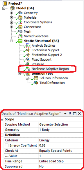
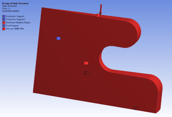
Let’s take a look at a simple example. This is a wedge portion of a circular hyperelastic part, subject to a pressure load on the top surface. Other boundary conditions include a fixed support on the bottom and frictionless supports on the two cut faces of the wedge.
For this case, the nonlinear adaptive region is the entire part.
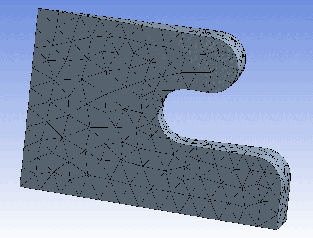
The initial mesh was setup as a default mesh, although note that for 3D models the nonlinear adaptive capability requires a tetrahedral mesh up through the current version, 2019 R2.
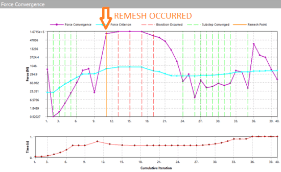
Prior to solving with the nonlinear adaptive region included, this model fails to converge at about 56% of the total load. With the addition of the nonlinear adaptive region, the model is automatically remeshed at the point of excessive element distortion, and the solution is able to proceed until the full load is applied. The force convergence graph has a solid vertical orange line at the point where remeshing occurred. The method can result in multiple remeshing steps although in the sample model shown here, only one remeshing was needed.
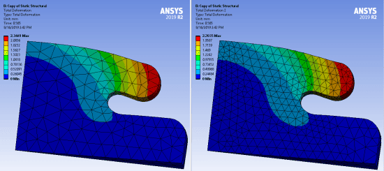
The image on the left, below, shows the original mesh at the last converged substep before remeshing occurred. The image on the right is the first result set after remeshing was completed.
The tabular view of a result item will show in the last column if remeshing has occurred during the solution.

Here is the final deformation, for the full amount of pressure load applied on the top surface.
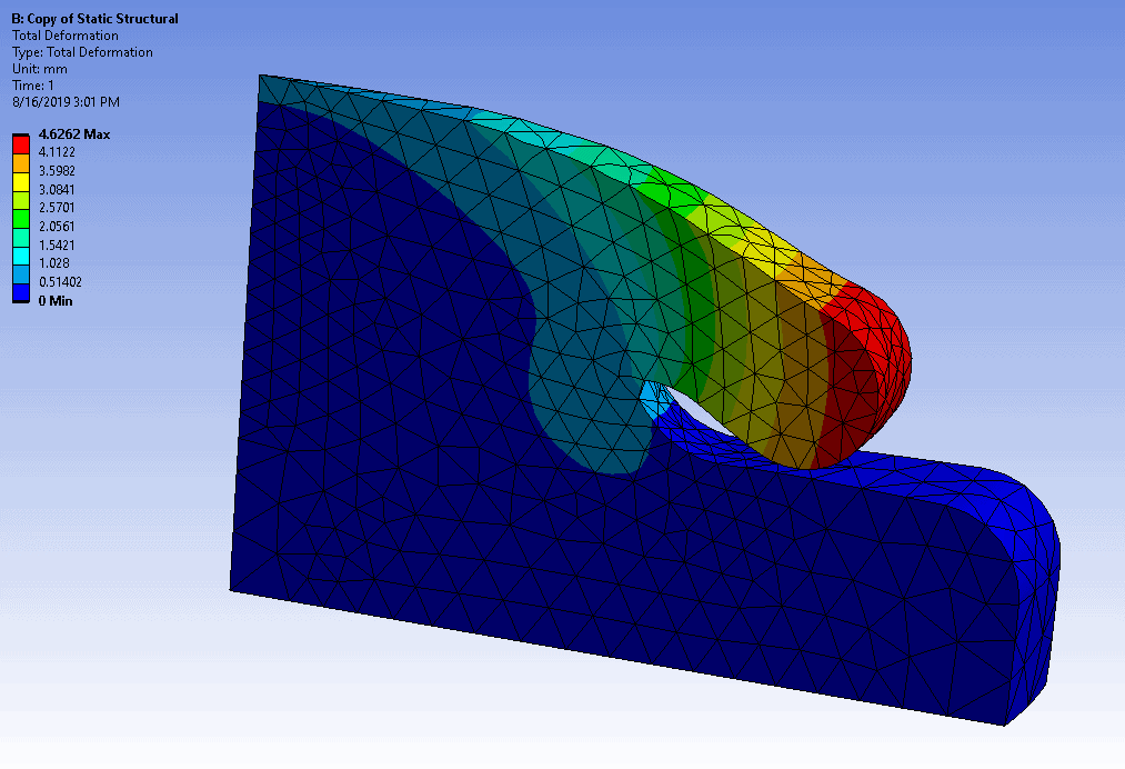
Next, let’s take a look at the nonlinear adaptive region capability in more detail.
First, multiple substeps must be used for the solution. If we are performing a nonlinear analysis, this will be the case anyway. Second, Large Deflection needs to be turned on in the Analysis Settings branch. Also, results must be stored at all time points (note that time is a tracking parameter in a static analysis, but all static as well as transient results in ANSYS Mechanical are associated with a value of ‘time’).
There are several restrictions on features that CAN’T be in the model, such as cyclic symmetry (hence the frictionless support BC’s on the simple model shown above), Auto Asymmetric Contact, Joints, Springs, Remote Forces and Displacements, etc. Also certain material properties are excluded, such as Cast Iron plasticity and Shape Memory Alloy. Also, as mentioned above, for 3D models, the mesh must be tetrahedral. For a full listing of these restrictions, refer to the ANSYS Mechanical User’s Guide. A search on ‘nonlinear adaptive’ will take you to the right location in the Help.
Nonlinear Adaptive Regions can be scoped to 3D solid and 2D bodies, or to elements via a Named Selection.
In the Details view for the Nonlinear Adaptive Region, the main option to be defined is the Criterion by which remeshing will be initiated. There are three options available in Mechanical: Energy, Box, and Mesh.
The Energy criterion checks the strain energy of each element within the Nonlinear Adaptive Region. If the strain energy is above a criterion, remeshing is triggered. The input is an energy coefficient between zero and one, and is a multiplier on the ratio of total strain energy of the component divided by the number of elements of the component. Recommended values are 0.85-0.9. A lower coefficient will tend to cause remeshing to be more likely.
The Box criterion defines a geometry region based on a coordinate system and bounds relative to that coordinate system. Elements in the Nonlinear Adaptive Region whose nodes have all moved within the box will be remeshed. The idea is that if it’s known that elements will be highly distorted as they move into a certain region, we can ensure that remeshing will occur there.
The Mesh criterion allows us to specify that remeshing will occur if mesh quality measures drop below certain levels as the mesh distorts. For 3D models, the available measures are Jacobian Ratio and Skewness. These are described in the Mechanical User’s Guide in the section on Nonlinear Adaptive Region.
In the example shown above, the Energy criterion was used with an energy coefficient of 0.85.
There are some things to be aware of when you are trying to implement a Nonlinear Adaptive Region to help overcome convergence difficulties. First, if any of the restricted features mentioned above are included in the model, such as remote displacements, it’s not going to work. Therefore, it’s important to review the list of restrictions in the Help and make sure none of those are applied in your model. Second, ‘buckling’ or element distortion due to an unstable structure is not a behavior that Nonlinear Adaptive Regions can help with. The Nonlinear Adaptive Region capability is more suited to problems like hyperelastic seals being compressed or objects that are undergoing a high degree of bending (but not snapping through).
Also, a coarse mesh that distorts may not produce a usable remesh. The remeshing step may occur, but the simulation may not be able to proceed beyond that and stops with an error in element formulation error. More mesh refinement may be needed in this case.
As a further word of caution, self contact problems may not work very well within the context of Nonlinear Adaptive Regions. If self contact is needed, consider splitting the bodies into multiple parts to avoid self contact.
There are some other considerations for the method as discussed in the Help, but hopefully the guidelines and recommendations presented here will allow you to filter potential applications appropriately and setup models that can take advantage of the Nonlinear Adaptive Region capability. We have a short animation which shows the remeshing step in the sample model.
If you have nonlinear static structural models with convergence difficulties due to excessive element distortion, please consider using this method to help you get a fully converged solution.
Here is a video to help everyone visualize:
As this video shows, adaptive meshing is a game changer for many complex large deflection problems and has opened a whole new category of simulation that can be done in Ansys Mechanical.


