
Finite Arrays
In addition to explicit modeling of finite arrays in Ansys HFSS, there are three other methods based on using unit cells. To learn more about the unit cell, please see part 1 of this blog.
In part 2, I will introduce and compare these 3 methods (1) Finite array defined using the array setting in unit cell, (2) Finite Array using Domain Decomposition Method (FADDM), (3) 3D component arrays (Figure 1). Please note that that the method 3 requires HFSS 2020R1 or newer.

(a)

(b)

(c)
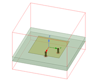
Figure 1. (a) Unit cell, (b) FADDM, (c) 3D component array.
Finite Array using Unit Cell
After defining a unit cell (Figure 1a), you may simply define the number of elements, the spacing between them, and the scan angle. The assumption is that there is no mutual coupling, every element has the same radiation pattern and the same excitation. This is a good approximation for large arrays (10×10 or larger). This method may not be accurate enough in some cases, for example for a small number of elements; and when the antenna elements have main beams toward the angles that are close to the plane of the array and toward the other elements, causing a higher level of mutual coupling. However, smaller arrays won’t require as large of a compute resource as a large array.
The advantage of this method is its simulation speed. It requires the minimum memory and time to provide a quick array simulation. To define the array (after running the analysis for unit cell), right-click on Radiation from the Project Manager window. Select Antenna Array Setup, and then Regular Array Setup. In the Antenna Array Setup under Regular Array type, define the location of the first cell, the direction, the distance between the cells and number of cells in each direction.

(a)

(b)

(c)
Figure 2. Steps to define a finite array, (a) Antenna array setup, (b) & (c) Regular array setup.
Finite Array using Domain Decomposition Method
General Domain Decomposition (DDM) for a single domain provides a way to reduce memory requirement, however, it does not reduce the meshing time for large explicit arrays. Using Finite Array DDM (FADDM) addresses this shortcoming. The FADDM bypasses the adaptive meshing stage by duplicating the mesh that was generated for a unit cell. While the unit cell is used to create the mesh, the assumption of uniform excitation is no longer present. Each element in FADDM can have different magnitude and phase and is individually modeled, however, the mesh created in the unit cell is used to generate the overall mesh, therefore, no CPU time is spent on generating the mesh. This can be seen in Figure 3, by linking the mesh of the unit cell to the FADDM, the mesh is copied, and no mesh refinement will be needed. You may compare it with the explicit array of the same size (Figure 3(c)) where the entire array has to be meshed and mesh refinement will be necessary for adaptive meshing. This can be a huge simulation time saving when the array size is large.

(a)

(b)

(c)
Figure 3. (a) Mesh from a unit cell, (b) mesh linked to FADDM, (c) explicit array mesh.
To create FADDM from unit cell, create a new HFSS design. Then copy the unit cell into the new design. In the Project Manager window, right-click on Model and choose Create Array, as shown in Figure 4. This opens the window that allows user to define the number of elements of the array along the lattice directions. By selecting “Active Cells” tab, user can define where active, passive and padding cells are located. This gives the user a means of creating different lattice shapes.
Please note that padding cells defined in the General tab represent the size of vacuum buffer surrounding the array. They are not visible to the users but are included in the FADDM simulation. The same mesh from the unit cell simulation is duplicated to padding cells (Figure 5). It is also possible to add padding cells in the Active Cells tab, and those cells are also invisible, but can be used to create the array lattice of the desired shape (Figure 6).

Figure 4. The steps to create a DDM array, the Padding Cells are used to create the vacuum box and are invisible to the user.

Figure 5. The FADDM needs a padding cell to create a vacuum box around the design. The padding cells are invisible to the user.

(a)

(b)
Figure 6. (a) Padding cells can be used to create a lattice, (b) the lattice created does not show the padding cells.
The next step is to link the mesh to the unit cell. First, an analysis setup should be created. Choose Advanced Solution Setup. In the Driven Solution Setup General tab, reduce the number of Maximum Number of Passes to 1, as shown in Figure 7(a), then choose Advanced tab and click on Import Mesh (Figure 7(b)). Click on Setup Link. This is to link the simulation to the mesh of a unit cell. There are two steps needed here. First, choose the file or design that contains the mesh information (Figure 7(c)), second is to map the variables Figure 7(d). The last step to setting up the analysis is selecting Advanced Mesh Operation tab and selecting “Ignore mesh operation in target design” (Figure 7(d)). Now the array is ready and simulation can be run. You notice that adaptive meshing goes to only one pass. If in Setup Link window the option of “Simulate source design as needed” is checked (Figure 7(c)), then if a design variable that affects the geometry is changed, the meshing of the unit cell is repeated as needed. After the simulation is completed the elements magnitude and phases can be changed as a post processing step by “Edit Sources” (right-click on Excitations). The source names provided in the edit sources is slightly different than an explicit array (Figure 8)

(a)

(b)

(c)

(d)

(e)
Figure 7. Different windows related to setting up a linked mesh in FADDM.

Figure 8. Edit sources gives the ability to change the magnitude and phase of each element.
To compare the run-time and array patterns an example of circular polarized microstrip patch antenna of a 5 ´ 5 element array is shown in Figure 9 and Figure 10. The differences can be seen at angles away from the broadside angle. This shows how the edge effects are ignored in the unit cell approximation. Table 1 shows the comparison of memory and runtime for the three methods.
Table 1. Comparing run time and memory needed for a 5 x 5 array, explicit array vs FADDM.
| Elapsed Time (min:sec) | Memory (MB) | |
|---|---|---|
| Unit cell | 01:06 | 83.1 |
| FADDM | 03:17 | 81.4 |
| Explicit Array | 25:06 | 94.7 |

Figure 9. Comparison of the far-field patterns for LHCP (co-polarization) created using FADDM and unit cell array.

Figure 10. Comparison of the far-field patterns for RHCP (cross-polarization) created using FADDM and unit cell array.
Finally, we compare the co-polarization pattern with an explicit 5 x 5 element array for scan angles of 0 and 30 degrees in Figure 11 and Figure 12, respectively.

Figure 11. Comparison of far-field LHCP created by explicit array vs. FADDM.

Figure 12. Comparison of scanned far-field LHCP, scan angle of 30 degrees.
3D Component Array
In 2020R1 the option of 3D component array was added. This option provides a means of combining different unit cells in one array. The unit cells are defined and imported as 3D components. To create a 3D component unit cell, define each type of the cells in a separate HFSS design, run the analysis, then select all objects in the model. In the Model ribbon, click on Create 3D Component, assign a name (no spaces are allowed in the name), add any information you like to add such as owner, email, company, etc., then click OK. Once all the 3D component cells are created, create a new HFSS design for the 3D component FADDM.
The next step is to create Relative CS for each of the 3D component elements in the HFSS design that will contain the array. For this step you need to plan the array lattice ahead of time, so the components are placed in the proper locations (Figure 13). Overlap is not allowed.
The unit cells should have the followings:
- Identical dimensions of the bounding boxes
- Identical Primary/Secondary (Master/Slave) boundary on the unit cells.
The generation of FADDM is similar to single unit cell array, except that when you select Model->Create Array, the window will be shown as 3D Component Array Properties (Figure 14). After choosing the number of elements and the number of padding cells, the unit cells window (Figure 15) will give you options of choosing one of the 3D component unit cells for each location of the elements in the lattice. The cells can be color coded. In the example shown in Figure 16 there are 3 components, the blank cell, the vertical cell and the horizontal cell. The sources under Edit Sources window are also arranged based on the name of the 3D component cells. At this point there is no option of linking the mesh. Therefore, the number of passes for adaptive mesh should be set to a number that is appropriate for getting a convergence.

Figure 13. 3D component unit cells are arranged to create a 3D component array.

Figure 14. The 3D component array can be created the same way as creating FADDM using a unit cell.

Figure 15. The unit cells are color coded for easier lattice creation.

Figure 16. The result of lattice created using 3D component array.
Conclusion
Unit cell and Finite Array Domain Decomposition are excellent options for simulating large finite arrays within a reasonable runtime and memory requirements. The 3D component finite array is a nice added feature in 2020R1 that now provides a way to combine unit cells with different geometries in one array.
If you would like more information related to this topic or have any questions, please reach out to us at info@padtinc.com.


