
With Icepak now falling under the umbrella of Electronics products in the Ansys Pro Premium Enterprise licensing scheme, it is easier than ever to obtain conjugate heat transfer simulation results without a dedicated Fluids license. Because of this, we have received multiple requests regarding methods to transfer Icepak’s results to a workbench environment for more accurate thermal and Mechanical results. So, without further ado, I will outline the procedure for four different methods along with their general use-cases.
1: Temperature from Classic Icepak
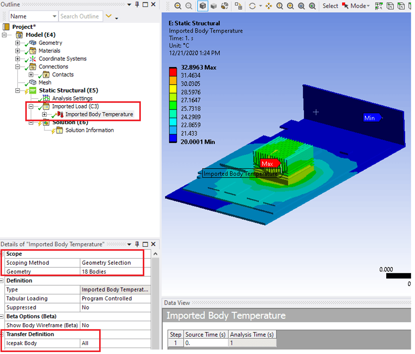
The first, and most straightforward, method is simply transferring body temperature directly from the Icepak (Classic) workbench application. This may be the preferred method for the majority of use-cases where getting thermal CHT results into a mechanical project is the goal. The Icepak node needs to be solved as normal, and then the solution can simply be dragged over to the setup node of another project, such as steady state thermal or static structural. Once this has been linked and updated, the transferred body temperatures are accessed through an “Imported Load” folder where the temperatures for individual bodies can be mapped over. The benefits are that as long as the Icepak simulation is set up as needed, you won’t need to resolve anything on the thermal side, and there is no extra manipulation of data required on the user’s end.


2: Heat Transfer Coefficients from Classic Ansys Icepak
The second method that sits natively within Workbench involves mapping heat transfer coefficients onto surfaces. This of course means that the thermal problem must be solved again, but it does provide extra accuracy over uniform HTC approximations, and some extra flexibility for recalculating body temperatures that result from changing power input conditions. This might be the desired approach if you are working with a forced flow and are looking at thermal stress results across a range of CPU loads, for example. HTC coordinate maps can be exported from Classic Icepak through the “Full Report” command with “Only summary information” disabled.

The complicating factor for this method is that the file format and information is not compatible with Workbench for External Data mapping in its default form.
I wrote a simple python script for this purpose – it reads in the HTC coordinate data, makes it all positive, rewrites it as a CSV, and adds the necessary reference (ambient) temperature column. It is important to note here that there can be an error in reported HTC sign from Icepak. This is because the sign is determined by the direction of heat transfer, which is reported without consideration to the solid body surface normal direction. So, for entirely convex shapes, the sign will be correct, but for more complicated structures like heatsinks with surfaces facing every which way, the signs will be inconsistent. Once this is done, each column needs to be correctly associated in the external data definition and then mapped to the setup of your thermal simulation. In Mechanical, this causes an Imported Load to show up under Analysis, which you will then insert a Convection Coefficient into. This can be scoped to individual faces, which should of course be included with those chosen when exporting from Icepak.


For reference, the python script may look something like:
############################################
import numpy as np
import sys

##Usage is 'python HTCCleanup.py inputfilepath AmbientTemperature'
inputfile = sys.argv[1]
Temperature = float(sys.argv[2])

#Bring in Icepak data file as argument
data = np.loadtxt(inputfile,skiprows=25)

#Make all HTCs positive
data[:,4] = abs(data[:,4])

#Create and append a reference temperature column
temparray = np.ones([len(data[:,0]),1])*Temperature
data = np.append(data,temparray,axis=1)

#Write to file
np.savetxt('ProcessedReport.csv',data,delimiter=',',fmt='%.5e',header='Node#, x, y, z, HTC, TRef')
############################################
3: Temperatures from EDT Icepak
The electronics desktop version of Icepak is a newer and, in my opinion, a more user-friendly environment for Icepak simulations. However, since it does not integrate directly with Workbench, mapping over result data for further structural simulation is not as straightforward. Luckily for us, other users have already addressed this obstacle via an ACT extension!
This is the “Write Thermal Loads” extension that can be downloaded for free from the Ansys App Store (https://catalog.ansys.com).

Once loaded, the interface looks like this:

Basically, this is a guided wizard that will export an external data file with coordinate defined temperatures according to the EDT bodies you select with the Wizard. The wizard also generates some workbench script files that can be used to automate the import process, but the most important part to know is that the temperature data file is brought in through External Data in essentially the same way as the aforementioned HTC file. For those who are familiar with the EDT environment and want to take thermal results straight into a structural analysis, this is the preferred approach.
4: HTCs from EDT Icepak
This is perhaps the most awkward (and advanced) workflow, but it provides the same flexibility as with Classic Icepak HTCs, without the potential error in HTC sign, and with the benefit of working in the EDT environment. The portion of this flow most likely to contain errors is generating the HTC data file, as we must make use of a normally inaccessible operation in the Field Calculator. After solving an Icepak project and generating results, we should first create a face list including all of the convection faces of interest – this is done by selecting those faces in the GUI and then using the Modeler > List > Create > Face List to generate this face. Once the list is created, open the field calculator (Icepak > Fields > Calculator), and then perform the following steps:
- Input > Quantity > Heat Transfer Coefficient
- Input > Geometry > Surface > Face List
- Scalar > Mean > Undo (ONE TIME)
- Output > Write
The single undo operation grants us access to the intermediate step where HTC data is accessible as a “SclSrf: SurfaveValue(Surface,HTC)” datatype, and can also be accessed by performing undo after any other scalar operation on a scalar field definition. (such as integration over a surface or body or a min/max calculation, for example)
The .fld file produced with the write operation is close to usable in workbench, but still must be slightly reformatted and appended with a reference temperature column. I would suggest a python script that is very similar to the one used for Classic HTCs.
One thing to note is that these files generated by EDT can end up being much larger than you may expect. This is because the field calculator essentially forms a list of all the surface elements on the surfaces you have specified, decomposes them into triangular elements if necessary, and then reports the HTC value of that triangular element at each connected corner node. So, you end up with 3 times as many data entries as you have surface elements, multiple HTCs reported for each node that touches more than one surface element, and a correspondingly large file for fine meshes on complicated geometries. Still, Workbench will interpret this whole thing fairly well, and you should end up with a good HTC map to make use of in Mechanical.


