Using a Table for Transient Actions in Flownex

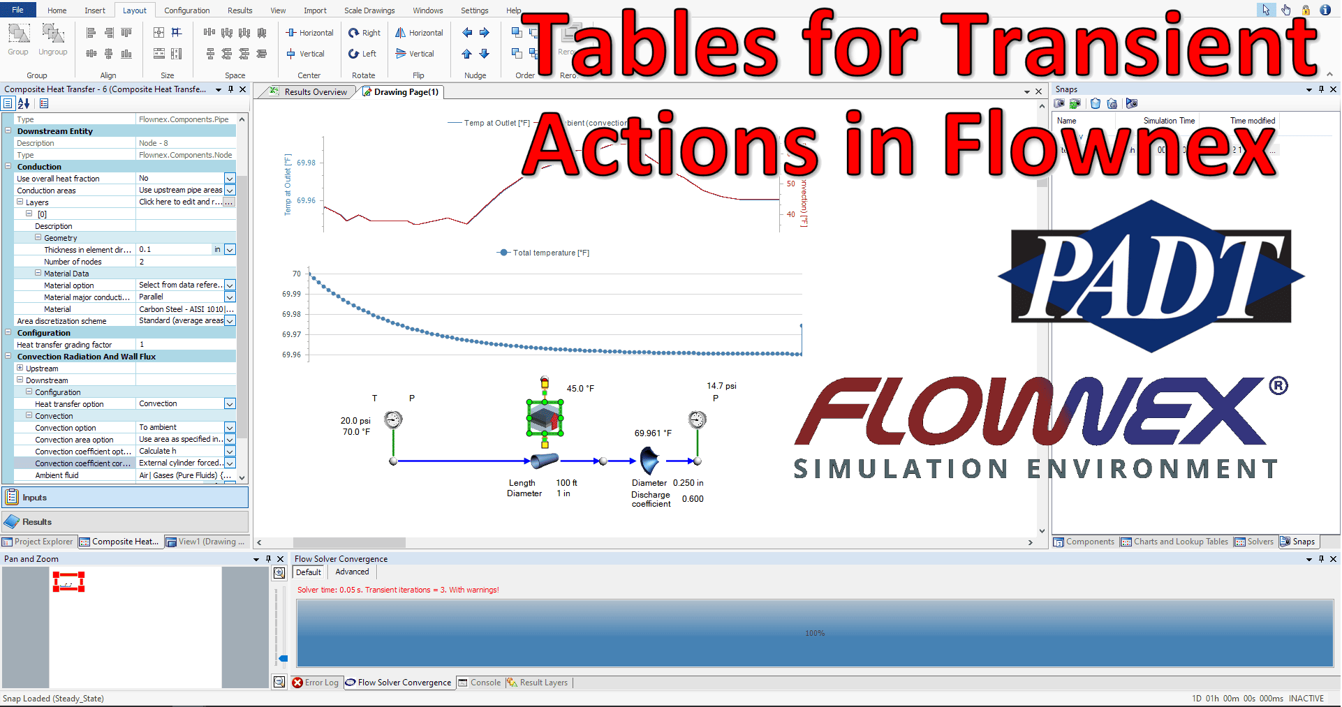
Happy New Year! Today I want to show how we can easily use the new “Table” option to vary an input to our transient simulation. In this demo I am using Flownex version 8.12.8.4472.

Building the Fluid Network

If you’re most interested in how to implement the table for the transient inputs feel free to scroll past these next few sections. We’re going to go over the basic network building steps in case the information is found useful.

I chose to use a very simple network of a pipe with water flowing through it exposed to ambient air. We’ll use commercial steel for the pipe, with an inner diameter of 1 inch and a length of 100 feet. In my mind I’m pretending this is an irrigation line and as such I will add a restrictor at the end to represent something like a sprinkler head.

Heat Transfer to Ambient

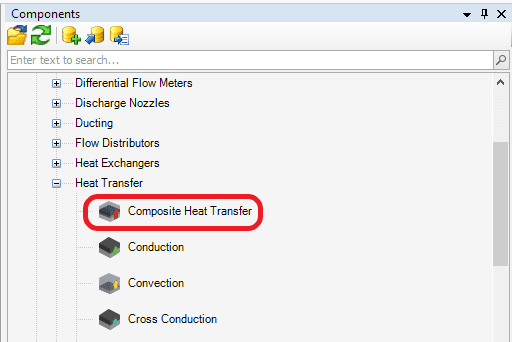
The next thing we’ll want to do is model the heat transfer to ambient by way of a Composite Heat Transfer element. I have the upstream side connected to my pipe and will take advantage of that when getting areas for conduction and convection.

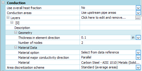
We can change the conduction areas drop-down to “use upstream pipe areas” and add an appropriate thickness and material type:

For upstream convection (water side), we can choose an appropriate correlation for calculating the convective heat transfer coefficient. Notice where we are obtaining inputs from the area specified in conduction and from the attached flow component. This saves us the effort of redundant calculations/inputs.

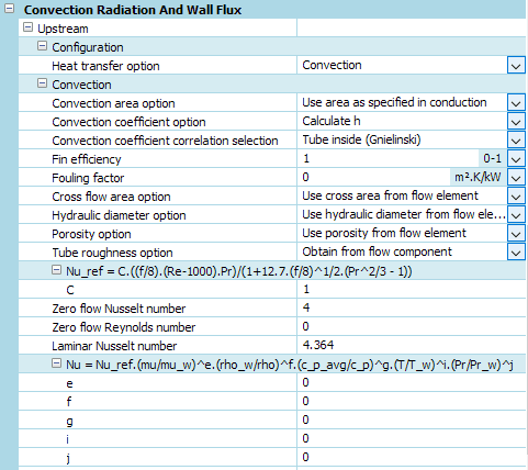
On the downstream side (air) we will set the composite heat transfer element for convection to ambient. For this set of inputs I still use the area specified in convection and then choose appropriate calculation operations for natural convection.

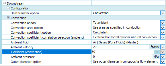
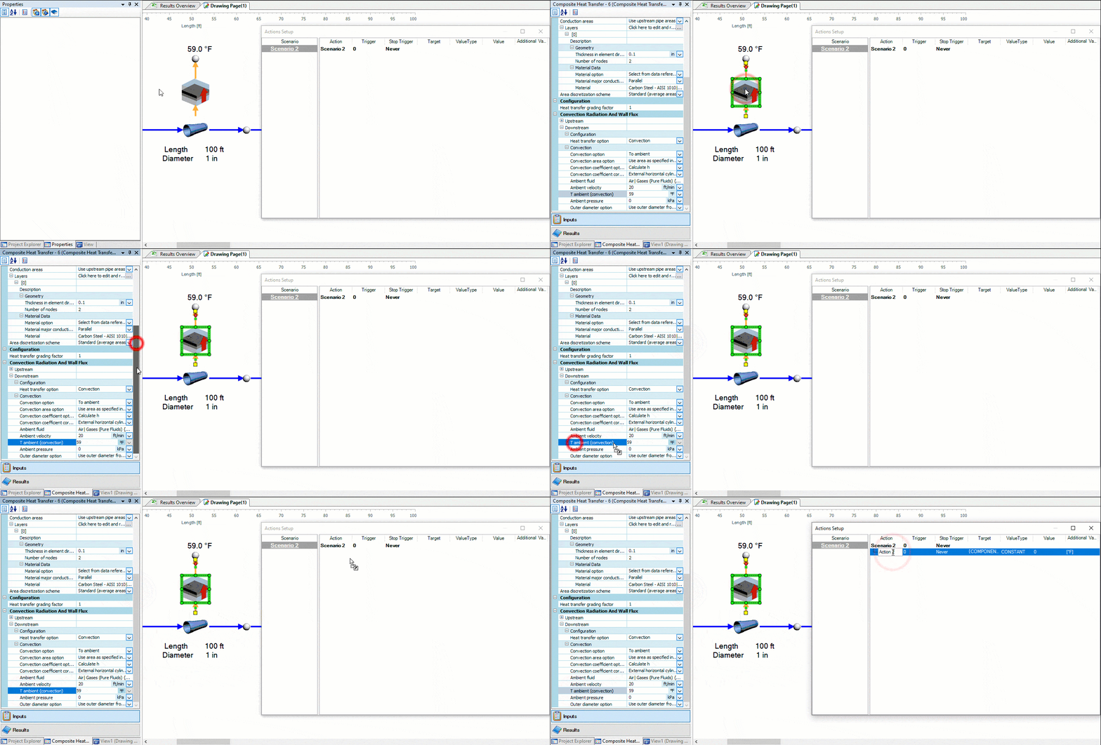
The key input we will be manipulating in the transient simulation is “T ambient” from the downstream composite heat transfer component. I will drag this property onto the canvas so we can easily monitor it during the run.

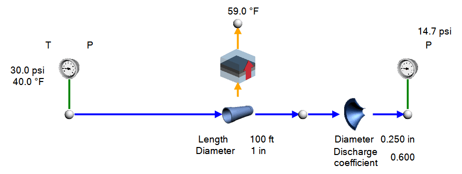
Setting up the Transient Scenario

What I’d like to model transiently is the effect of the changing ambient temperature on the temperature of the water in the pipe. To create a new transient scenario we go to the Configuration ribbon, click on actions setup, then in the Actions Setup Window we will right-click and “add scenario”

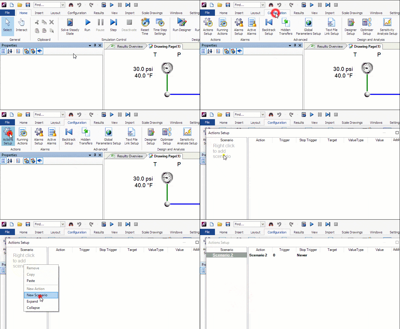
Since we will be manipulating the ambient temperature we will want to drag and drop this input into our newly created transient scenario as an action:

Using Table for Transient Action

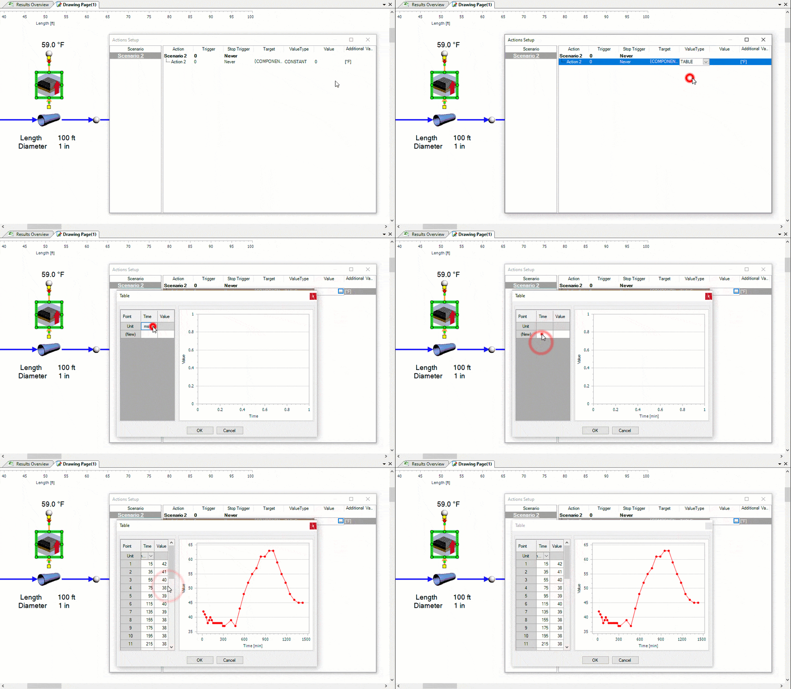
We should choose “Table” under ValueType if we want to use the new Table option for varying our input transiently. I am going to use weather data for earlier this week for Phoenix, Arizona as my table of inputs. To make things easier I have converted the time to minutes after midnight.

Time	Minutes After Midnight	Temp [°F]	Humidity	Wind	Wind Speed	Condition
12:15 AM	15	42	83 %	ESE	6 mph	Fair
12:35 AM	35	41	86 %	E	5 mph	Fair
12:55 AM	55	40	86 %	E	5 mph	Fair
1:15 AM	75	38	89 %	SE	7 mph	Fair
1:35 AM	95	39	87 %	SE	9 mph	Fair
1:55 AM	115	40	84 %	ESE	6 mph	Fair
2:15 AM	135	39	85 %	SE	6 mph	Fair
2:35 AM	155	38	87 %	SSE	7 mph	Fair
2:55 AM	175	38	87 %	SSE	9 mph	Fair
3:15 AM	195	38	87 %	SE	7 mph	Fair
3:35 AM	215	38	86 %	ESE	7 mph	Fair
3:55 AM	235	38	84 %	ESE	7 mph	Fair
4:15 AM	255	38	86 %	NE	7 mph	Fair
4:35 AM	275	38	85 %	E	8 mph	Fair
4:55 AM	295	37	87 %	E	5 mph	Fair
5:50 AM	315	37	81 %	ESE	8 mph	Fair
6:47 AM	407	39	75 %	ESE	8 mph	Fair
7:50 AM	470	37	81 %	E	6 mph	Fair
8:54 AM	534	43	70 %	ESE	5 mph	Fair
9:50 AM	590	48	54 %	SE	7 mph	Fair
10:50 AM	650	52	50 %	SW	3 mph	Fair
11:50 AM	710	55	44 %	CALM	0 mph	Fair
12:50 PM	770	57	41 %	WNW	3 mph	Fair
1:50 PM	830	61	36 %	WNW	5 mph	Fair
2:50 PM	890	61	36 %	CALM	0 mph	Fair
3:50 PM	950	63	32 %	SW	3 mph	Fair
4:50 PM	1010	63	32 %	CALM	0 mph	Fair
5:47 PM	1067	59	39 %	S	5 mph	Fair
6:47 PM	1127	55	44 %	VAR	5 mph	Fair
7:47 PM	1187	52	58 %	SSE	3 mph	Fair
8:47 PM	1247	48	71 %	E	5 mph	Fair
9:47 PM	1307	46	76 %	ESE	8 mph	Fair
10:50 PM	1370	45	81 %	ESE	6 mph	Fair
11:47 PM	1427	45	81 %	ESE	7 mph	Fair

The next step is to simply copy and paste or drag and drop our series of values into our new table.

Let’s run a transient and see how it behaves! Note that I’ve added an increment plot showing the temperature profile as a function of linear length of the pipe. I also modified my inlet boundary condition so that we’d have a more observable change in temp over the length of the pipe.

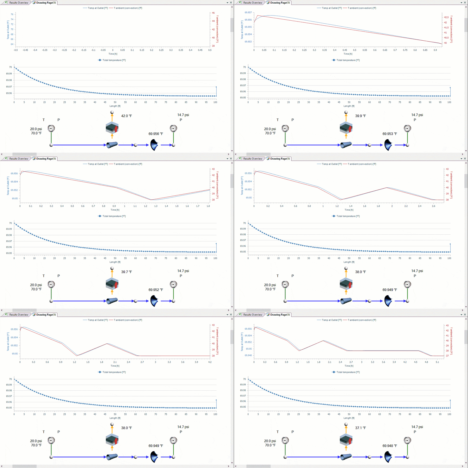
Although the outlet temperature stays relatively constant, if we look at the change overlaid with the changing ambient temperature we see the expected correlation. An interesting next step might be to incorporate the wind speed data and model the external convection as forced convection where we vary the wind speed according to our table.