Do you hear that sound? It’s the celebration of all my adoring fans celebrating a long-awaited blog post! I figured having “create new blog content” on my quarterly review for the past 32 quarters was impressive, but 33 was just unacceptable. So here we are. In an attempt to trick myself into routinely writing something, I’m starting what I’m calling “hold my beer” type of articles where a quick write-up of a work-around, fix, new feature, etc is discussed. Basically, if someone says some task is too difficult, tedious, etc… hold my beer, cuz I’mma fix that for you.
All right, first topic… can you create a spatially varying material property definition. I sure hope you’re not using a stand-up desk… because the answer is yes. This process is more commonly used for lattice optimization (validating the variable field map), simulating composites (creating a map of degradation factors), or the newer short fiber composite workflow (which is extremely cool…check it out…caution: potential foreshadowing). Behind the scenes, we accomplish this by using field variables. While I listed some common/standard field variables above, you’re more than welcome to define your own variable for use in mapping. These field variables are usable for most common material properties…to show I’m not lying, here’s a documentation link:
The way these field variables work is I define my material properties (see documentation above for supported materials) vs. a field variable. I then map that field variable onto my elements, and they then look up what the material is. Brilliant!
Because I just had an MRI, let’s start with a hypothetical situation where I want to run a simulation where I’m converting MRI data into linear elastic behavior. The first stop on our journey is Engineering Data:
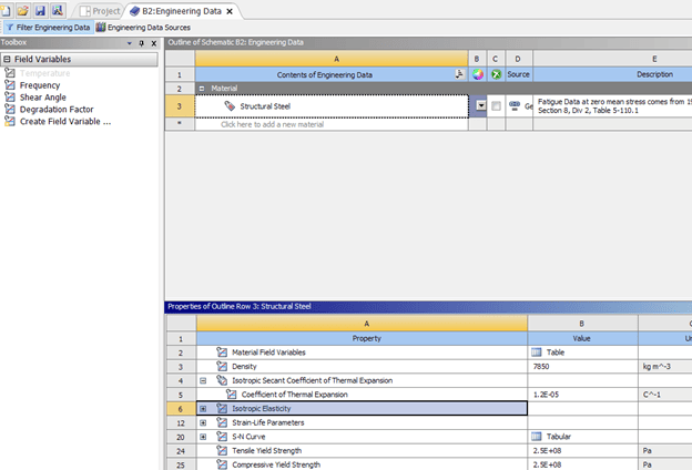
Note, in order for ‘field variables’ to show up I actually have to click on the material model in the outline row. If I hadn’t clicked on ‘isotropic elasticity’ then I wouldn’t see ‘field variables’. For this I’ll just double click ‘create field variable’:
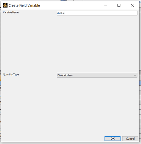
The name here doesn’t need to match. I’m doing that just for my own sanity. Ultimately we’re just mapping information from a point cloud to the mesh. After I hit ‘ok’ in that image I’ll now see:
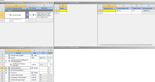
So now I can define two dvalue lines, which could then have different temperature-dependent effects, and fill out the young’s modulus definition:


So I’ve now defined for dvalue=100, E=2E11 prxy=.3 and for dvalue=200, E=1E11 prxy=.27.
Super easy so far. I have defined a material model that will create a tabular representation modulus. Now we go to External Data to read in a CSV file which will map the field variable onto my mesh. The benefit here is that I can mesh my model however I like, and it’ll still perform the map.
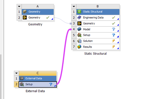
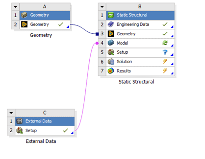
Note that external data can map many different things. Because we are mapping material information we need to connect it to the ‘model’ cell. Otherwise, if we had spatially dependent boundary conditions we could link it to the setup.
Going into External Data:
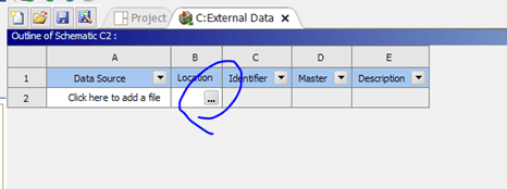
Select that to then browse to the CSV file (oh, forgot to say you need to save that excel file as a CSV):
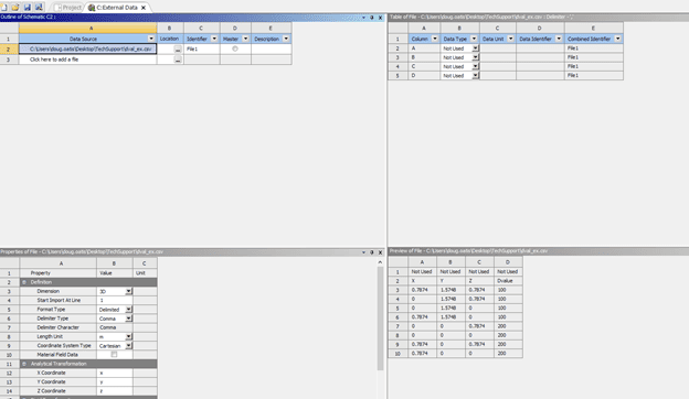
I now need to set some controls for how the file is read (bottom-left corner) and what the columns mean (top-right) which will generate a preview (10-rows only, bottom right).
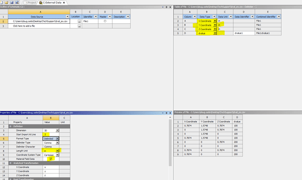
First select the ‘material field data’ which allows you to access the field data present in Engineering Data. Then specify the length (I took all my measurements in inches). Then, specify your column headers to be x/y/z/dvalue. Then verify that everything looks right in the preview…and finally toggle the option to start the import at line 2 (we don’t want to read the CSV header as mappable data).
All done, update things on the project page and open Mechanical (note, you can do this after you’ve already built a model, as shown I’m building it from scratch…just drag/drop the connections and ensure that everything is properly updated on the project page):
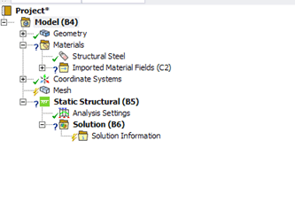
Now in Mechanical, I’ll see an ‘imported material fields’ item:
Scope the material field object to the body you want, right-mouse on it and update (this will mesh the body and perform the map):
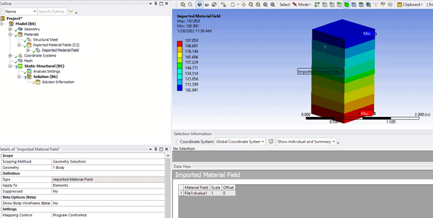
Reason it isn’t showing 100-200? This is mapped to the elements while the keypoint measurements were on the nodes (I built the CSV by just copying the x/y/z location of all my keypoints to excel and then defining a variation in the y-direction). So elements on the boundary will have a gradient and not be at 100 or 200…so this is correct.
Next, you want to look at the mapped values…which is easy! Insert a material plot into the plot branch, tada:
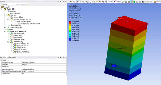
Lines up with the engineering data definition!
Behind the scenes you can dig into the input file to see what actually happened:
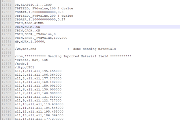
You can see lines 12581-12585 specify a tabular representation of isotropic elasticity. Then starting at line 12599 it’s starts applying a custom field variable to my elements using options from the initial-state/INISTATE family of commands. You don’t need to know any of this, I’m just showing how the sausage is made.
So, no need to cut your model up into a bunch of slices, fight carpal tunnel defining multiple material models and assigning them down your sliced up model, then threatening to quit when someone says that the spatial variations have changed. Field variables, external data, done.
I’ll take my beer back…


