Nonconformance in components or subsystems are important factors to consider when assessing the risk or reliability of a large or complex network. These may include component sizing, operating conditions, or simulating a worst-case scenario. It can be difficult to predict how variability in a system will impact key safety or efficiency parameters. Flownex is capable of performing a sensitivity analysis to determine the systemic impact of perturbations, variations in component specifications, or design outputs. or Monte Carlo analysis can help us define the effect of these changes. We will walk through how to perform a sensitivity analysis as well as a Monte Carlo analysis to determine the effect of varying component properties. We will be using Flownex version 8.14.1.4845 in this example.
Introduction
This example re-visit the completed low-pressure feedwater heater from tutorial 21. Our goal is to determine how the mass flow out of the system is affected by variations from the nominal design specifications. Initially, perform a parametric study by varying diameter of the pipes feeding water into the system from the condensate extraction pump (CEP). Then, we will vary the pipe roughness in a second parametric study. Finally, we will setup a Monte Carlo sensitivity analysis to vary both input variables between specified values with a normal probability distribution.
Parametric Study Setup
First, we will setup a sensitivity analysis by clicking on the sensitivity analysis setup button in the configuration ribbon. A new sensitivity analysis can be added by right clicking in the top pane. We will add a single input to the sensitivity analysis by dragging our input variable into the lower left pane. First, vary the diameter of the condensate pipes.
We will start by creating a parametric study to uniformly iterate the pipe diameter between specified values. Enter 0.023m for the low value and 0.0275m for the high value (with a nominal value of 0.025m) using 25 runs. The nominal value is arbitrary with a single parameter. We will also drag the mass source from the node on the lower left into our results pane.
It is also possible to run multiple inputs and results in our parametric study. For this example, we will also choose to vary the pipe roughness between 20µm and 100µm (with a nominal value of 40µm). We will also choose 25 runs to vary roughness.
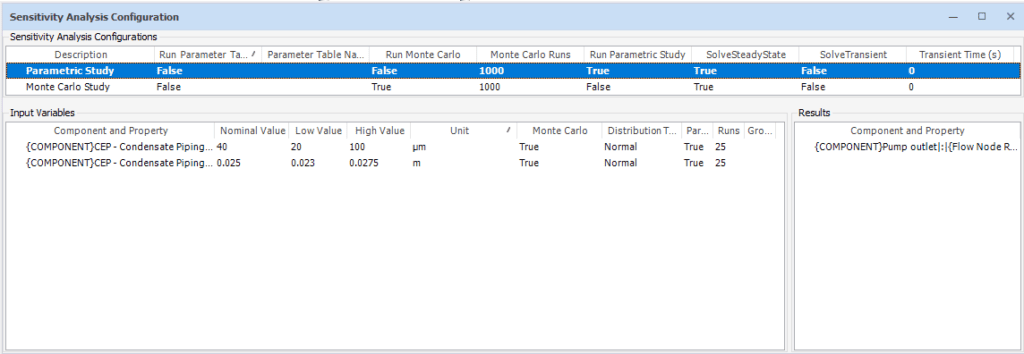
In this method, each independent variable will be used in a parametric study while other variables are assigned the nominal value specified. Each sequential study will be appended to the output file.
You may also choose to look at multiple output variables (e.g. mass flow and enthalpy at the outlet) when running a sensitivity analysis, simply by dragging additional outputs into the Results pane.
With our parametric study setup, we can navigate to the home ribbon to run the sensitivity analysis.

We will also run a second parametric study using the same method to determine the effect of the pipes’ roughness on the mass outflow.
Parametric Study Results
After running the parametric study, we can view the results in a plain text file using the “Sensitivity Analysis Results” button in the results ribbon.

The Sensitivity analysis results may also be exported to a report as described in the General User Manual. A screenshot of the results document is shown below.
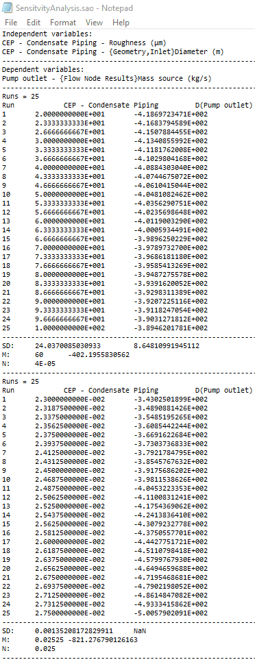
We can see data corresponding to our inputs and results from each run. This includes the mean, standard deviation and raw data for each run. We can also copy/paste this data into excel for visualization. Below is a plot showing the correlation between each input variable and total outflow (absolute value).
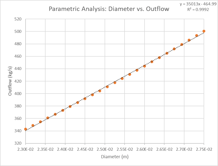
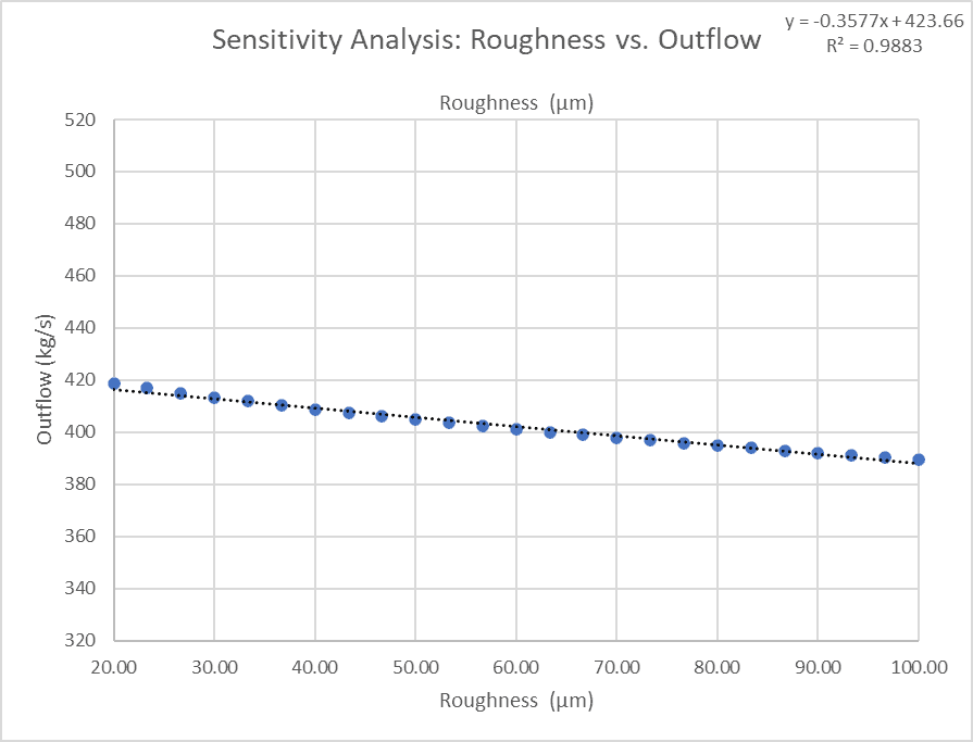
From the above graphs, the variation in pipe diameter will likely have a greater effect on the system than the roughness.
It is good practice to preselect parameters with the highest on the variable of interest. We can calculate the percent change of our output variables for each setup. We can calculate the ratio of percent change of our outputs to our inputs. We can calculate this ratio ([output %change]/[input %change]) for our roughness variation (0.054517) and our diameter variation (2.109503) to quantify the impact of each variable. It may also be important to consider the percent change in output if the expected ranges of operation (or tolerances) are known.
We can predict that varying the diameter should have a larger impact on the mass flow out of the system. For a more detailed model validation, additional input variables may be evaluated the parametric study, and only the variables with the highest impact would be elected for a Monte Carlo sensitivity analysis. determine if their impact is significant prior to running a Monte Carlo sensitivity analysis.
Monte Carlo Analysis Setup
Next, we will setup a Monte Carlo study using the same input parameters. A Monte Carlo sensitivity analysis will randomly vary each parameter according to the upper and lower limit of each variable and the probability distribution specified. We can determine how these parameters affect the outflow during normal system or lifecycle operation. We can drag both the roughness and diameter of the pipes into the input variables box and drag the value of our mass flow exiting the system into our results. Lastly, we will set the “Run Monte Carlo” option to “True” and the “Run Parametric Study” option to “False”. We will run this study for 1000 runs and will keep the Normal/Gaussian probability distribution (alternate probability distributions may also be specified for each input variable).

Monte Carlo Analysis Results
After running the sensitivity analysis, we can analyze the data. The header for the file lists the order of variables corresponding to each column. The results file will also list both input variables and results for each run. Below is a screenshot of the top of our output text file showing the number, roughness, diameter, and mass flow (negative values are exiting the system) for each run.
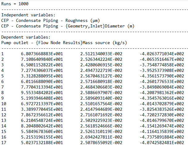
The mean and standard deviation of our outflow are located at the bottom of the sensitivity analysis results file.

We can see that our system has an average outflow of approximately 411.0kg/s with a standard deviation of 36.2kg/s.
Additionally, we can copy and paste the data from this analysis into Excel for visualization or post processing. The excel plots below show the roughness and diameter plotted against the outflow for all of the runs.
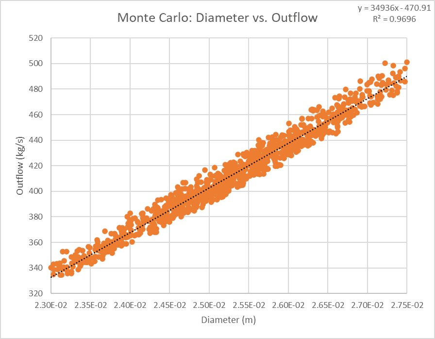
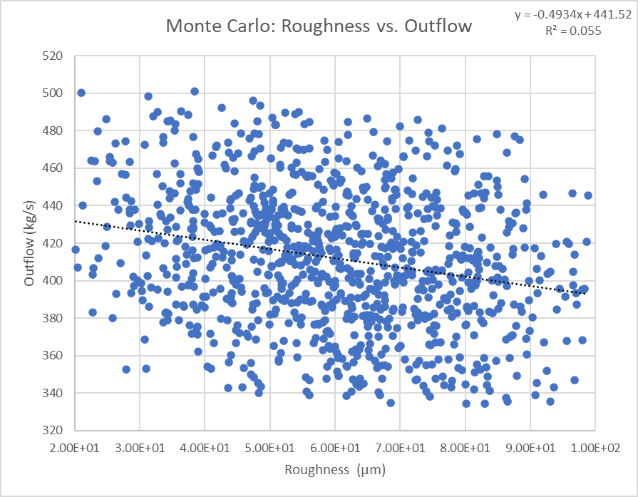
Now you have learned how to perform a sensitivity analysis using a parametric study for individual input variables or run a Monte Carlo sensitivity analysis using multiple input variables. This is a powerful design tool for evaluating design uncertainties.

