Taking Full Advantage of the Ansys Product Portfolio: 4-Way Multiphysics with Thermal Deformation Mapping to Ansys HFSS

The multiphysics workflows I typically deal with are thermal-electric in nature – after all, a big part of the value proposition for the Ansys EM Suite is that it includes and plays nicely with Ansys Icepak, which is vitally important when you need to understand how your electromagnetic analysis is affected when things get hot. However, there is another class of effects on EM solutions that is often overlooked for a variety of reasons: a relatively small effect on the end result, overall complexity of the solution process, or perhaps even a limitation on the Ansys licensing available at the time.

This effect is structural deformation of electrically active geometry, such that the electromagnetic solution reflects the influence of stresses pulling said geometry out of its ideal shape. A great example of multiphysics interaction. This deformation could be caused by mechanical loading (wind and/or insufficient support structure), body forces (like gravity causing a long antenna to droop), or even thermal expansion due to normal operation of the electrical device.

All these effects and analysis types are currently accessible in the Ansys product suite, but due to the prior reasons, they’re not often fully utilized for this type of multiphysics simulation. For instance, coupling a Static Structural solution type with HFSS requires someone knowledgeable in both the HFSS and Mechanical tools and all that those encompass. Model simplification, meshing, and boundary conditions can all require different skill sets for each physics type.

Once you throw in thermal physics via solid body conduction, you still have a mostly well-defined multiphysics workflow available, but again, you must at least be passingly familiar with thermal physics. Where things get more interesting is when that thermal solution is dependent on the detailed flow of fluid around your electrical device – say, the non-uniform natural convection of air around a high-powered antenna.

In that case, you might want to add a computational fluid dynamics solution into the mix as you may no longer be satisfied with making constant heat transfer coefficient assumptions on your antenna surface. Unfortunately, this level of Multiphysics – HFSS + Mechanical + Thermal + CFD is still niche enough that there are not many documented workflows that represent this full multiphysics process. All that said, this article is my current recommendation for how to approach this 4-way physics coupling and is taken from the perspective of someone who is:

• Already an HFSS/EM expert who wants to know more about their electrical design
• Needs better-than-constant-approximation heat transfer coefficients, but not necessarily perfect resolution on the fluid side of the problem
• Wants to learn as few simulation user interfaces as possible
• Has access to the equivalent of Electronics Premium HFSS + Electronics Premium Icepak (Or Electronics Enterprise) in addition to Mechanical Premium or Enterprise

Note that, as with any simulation, best practices regarding meshes, boundary conditions, etc, should be followed at each step of the analysis to obtain meaningful results. To make things convenient for any who are interested in following along, this walkthrough uses the ‘Waveguide Filter’ example project that is packaged along with EDT (Electronics Desktop). It can be located from File > Open Examples… > Icepak > Waveguide_Filter.aedt from inside EDT.

Steps Required to Set up a Multiphysics Workflow with 4 Different Solvers

So, without further ado, below is an outline of the steps that I take to enable this multiphysics workflow.

Step 1: In EDT, solve a coupled Icepak-HFSS model

This generates an initial set of temperatures, a fluid flow field, and a corresponding surface map of heat transfer coefficients. Follow the general instructions here: Using Ansys Icepak Results in Ansys Mechanical – PADT (padtinc.com) for exporting the HTC map from EDT Icepak and processing it into a form that is usable by Mechanical inside of Workbench. One note on the calculator step for section 4: HTCs from EDT Icepak – since writing that blog, I have found that the undo step is unnecessary. After selecting HTC and then your face list, simply use Output > Value button to obtain the needed ‘SclSrf: SurfaceValue()’ data type.

Step 2: Connect Multiphysics Models in Workbench

In Workbench, drag and drop your .aedt project file into the workspace to get an HFSS analysis type. This .aedt project file must ONLY contain an HFSS project, it cannot also contain Icepak. So, I suggest that you start with the .aedt project file from step 1., delete all unnecessary analysis types, and save it as a new HFSS-only project file.

Step 3: Open the new HFSS analysis block in your workbench project

Make sure you ensure that stress feedback and/or thermal feedback is enabled, as appropriate for the project goals.

1. For stress/deformation, only enable feedback for solid bodies that will be present in the Mechanical simulation.

2. For temperature feedback, only bodies with an assigned material property that includes a thermal modifier are enabled. So, make sure the materials are correctly defined inside of EDT first.

Step 4: Match Geometry and Coordinate Frames

The same solid body geometry in the same coordinate frame must be used in both Mechanical/thermal and HFSS cases for the bodies that are actually exchanging information. If you do not already have a separate geometry file, use the Modeler > Export option from inside your EDT project and generate a .stp geometry file. This can be used as the baseline for using Ansys Spaceclaim to add or remove other bodies that may not be significant for a given analysis. I.e., removing an air cavity that is needed for HFSS but not Mechanical, or adding a mechanical support structure that is not significant electrically.

Step 5: Create Workflow in Workbench

In the Workbench view with just your HFSS system present, build out the complete workflow like so:

1. Drag a Steady-State Thermal system onto the ‘Solution’ line of the HFSS system

2. Drag ‘Geometry’ from HFSS onto ‘Engineering Data’ in Steady-State Thermal
3. Drag a Static Structural system onto the ‘Solution’ line of the HFSS system (Same as step a)
4. Connect Engineering Data and Geometry from Steady-State Thermal to the corresponding items of Static Structural
5. Connect ‘Solution’ from Steady-State Thermal to ‘Setup’ of Static Structural
6. Connect ‘Solution’ from HFSS to ‘Setup’ of Static Structural
7. Right-click on ‘Geometry’ for Steady-State Thermal and use Import Geometry to bring in the .stp file from 4.
8. Add an ‘External data’ component system to the workflow, and drag ’Setup’ from External Data to ‘Setup’ on Steady-State Thermal
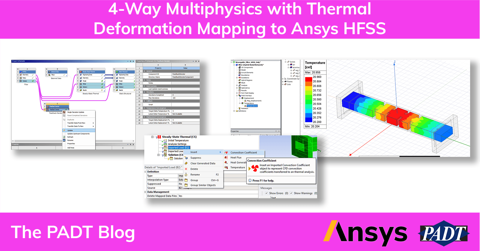
9. The end result should look like below. It is important at this time that the ‘Model’ of Steady-State Thermal and Static Structural not be attached, as we do not want/need the same mesh for both analysis types, and linking this can mess up the HFSS data transfer later on.

Step 6: Map Loads

Open the ‘Setup’ of External data, add the HTC map file (From step 1), then assign your data columns. Summarizing the prior mentioned article, you will need x/y/z point coordinates along with a heat transfer coefficient value and an ambient temperature value.

Once the data file is added and columns assigned, go back to the project view and right-click Update the External Data ‘Setup’, then ‘Update upstream components’

Step 7: Update the Thermal Model

Right-click > Update on ‘Setup’ for Steady-State Thermal. If HFSS was not already solved, this will solve the initial non-deformed isothermal case and enable future connection to the thermal/mechanical solvers. After the update is complete, open the Steady-State Thermal model:

1. Assign materials to each solid body as needed
2. On the ‘Imported Load’ for External data, right-click and insert a Convection Coefficient. Adjust the geometry scope so that it includes all the faces that were exported from the original Icepak thermal project. I suggest using the face selection filter and box select tool to grab everything.
   
   If external data was loaded properly, the Film Coefficient and Ambient Temperature fields should automatically populate:
   

3. For the Imported Load from HFSS, add a heat flux and scope it to all relevant surfaces:
   
   Note that you can Scale and Offset the imported load if desired:
   
4. With ‘Imported Load’ from HFSS still selected, go into Details > Export Definition and change ‘Export After Solve’ to Yes:
   
5. Add any result fields you want (Temperature, for example), and then solve the Steady-State Thermal problem. In the message section, there needs to be an ‘Info: Temperatures were successfully exported’ message:

Step 8: Repeat Step 7, but for Static Structural

For Imported Loads, there will be one from Steady-State Thermal and one from HFSS – the Steady-State Thermal connection should be fine by default. For HFSS, add either a body force or surface force with whatever object scoping is appropriate, and then make sure to enable ‘Export After Solve’ as before. As always, Mechanical boundary conditions will need to be applied to properly constrain the problem. Additionally, care must be taken such that HFSS requirements are not violated – e.g., port excitation surfaces must remain planar. Solve the Static Structural system and look for the same ‘Info: Structural results were successfully exported’ message.

Step 9: Enable HFSS Update

With Steady-State Thermal and Static structural each solved once, go back to the workbench project view and right-click on ‘Solution’ under HFSS > Enable Update:

Step 10: Update HFSS

Then, right-click ‘Update’ on the HFSS solution. This solves HFSS again with the updated temperature field and structural deformation.

You can now go back into the HFSS system and double-check the mapped temperatures, deformations, and general HFSS results via field plots.

Step 11: Repeat Until your Multiphysics Simulation converges

This update process can continually be repeated to iterate through solutions until converged. Or, drag the ‘Feedback Iterator’ component system onto the HFSS Setup line, set convergence criteria for delta temperature and/or displacement values and let it automatically loop through the process for you.

True Multiphysics Across Solvers Without the Hassle

This pretty much covers all the core pieces of this multiphysics workflow, and additional information on the stress-feedback loop with HFSS can be found in the online Ansys Help documentation (Ansys HFSS 2023 R1 – Ansys Workbench Integration Overview).

If you need any help with your complex simulations, please reach out to PADT for training, mentoring, or consulting. We have been living and breathing multiphysics since it was introduced in what is now Ansys Mechanical APDL over twenty years ago. We are here to help.