
As a typically mechanical / systems engineer, I am not exactly qualified to go through and list exactly what SIWave does and why you need it for any given situation (shoutout to Aleksandr, our actual expert, whose assistance has been invaluable for my simple example case). However, what I think I have grasped is that SIWave is just one of those Ansys tools where if you need it, you probably really need it. Where this becomes relevant to me is of course in a PCB thermal analysis. DCIR is typically the electrical half of this problem that is within SIWave’s expansive toolkit, though SIWave also contains some very easy-to-use thermal-oriented options for co-simulation with Icepak. I’ll admit that I have tended to somewhat dismiss this on my end, as I am already familiar with a couple more advanced thermal analysis tools, so why wouldn’t I just use these if I wanted to look at the thermal response of A PCB? Despite this, I have recently (begrudgingly) taken a more in-depth look at the thermal side of SIWave, and what I have found is that even if the settings available are a little more simplistic than I might always like, it really is incredibly accessible and provides some nice visualization capability. What’s more, it provides not only an easy path to view your existing thermal results in a full Icepak interface, but also serves as a great starting point if you need to analyze some more complex setups than Icepak.
So, having just been through much of this on my own, it seems like a great opportunity to share some tips and tricks for thermal visualization in both Ansys SIWave and Ansys Electronics Desktop (EDT) Icepak, see where each is strong relative to the other, and then perhaps even share some suggestions for using the SIWave solution as a starting point to take an Icepak PCB simulation to the next level!


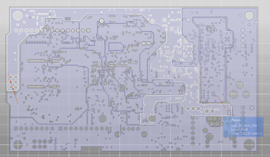
To start with, we need a SIWave DCIR project. A DCIR solution is required for providing thermal loads for a thermal solution. I am glossing over this, but basically, you need a PCB definition, a voltage source, and a current source. In the model I borrowed from Aleks, I am using these sources to push some current through one section of my PCB’s power layer and then referencing them to the ground layer. To complete the loop. This means that there are EM losses on both the ground layer and power layer.
For the first simulation, we’ll want to set a baseline temperature for our electrical material properties and make sure the toggle for “Export power dissipation for use in ANSYS Icepak and Mechanical” is enabled.
Now, we can set up an Icepak simulation! As I alluded to, the settings available within SIWave are somewhat primitive, although they do an overall good job of adhering to typical best practices. Our choices are basically using a board model without components and strictly modeling thermal conduction within that board, using a board model with components that includes explicit thermal convection to the environment, manipulating a mesh detail slider bar, and choosing the cooling regime used (natural vs forced convection). For this model, I’ll be using forced convection with surface components and “Detailed” meshing so that I have the most to look at, but obviously the exact settings will vary somewhat depending on your use-case. In 2021R2, the default SIWave-Icepak behavior will be to use EDT Icepak as the solver, however, we can choose to specify “Use Classic Icepak” in the simulation setup window. This determines which version of Icepak we have to use for additional postprocessing in as well, so I will leave “Use Classic Icepak” turned off.
The first method of visualization in SIWave is to simply right-click an Icepak simulation definition in the “Results” window and Display temperature.

This gives us a nice temperature contour on the outer surface of all the solid bodies considered during the simulation. If we stick with the top-down view, we can make use of a nice temperature probe that automatically displays at the mouse location. Once we rotate around into a 3D view with the middle mouse button or other view options, we lose this probe but of course, gain a nice graphical representation of the full geometry.

The second method is to use the View > Temperature Plots toolbar option, which gives us some more flexibility for viewing temperature through each layer.

Most commonly, we will probably be working with the XY cutting plane and then selecting the layer of interest from the drop-down menu so that we can see a plane through the entire PCB. For more precise control, we can also use the slider bar or input the exact plane-normal location to use for plotting.

One of the benefits of this approach is that we can use the other cutting plane definitions to get a cross-section view, along with whatever ECAD board elements we would like to plot. For instance, if we’d like to see more clearly how the temperature varies with depth underneath active components, or around via definitions, we can easily explore this, as in the image below.

Depending on your needs, this may be sufficient flexibility for observing the temperatures of interest, and the smoothly moving cut plane with the slider-bar position is certainly an easy way to get a sense of the board’s behavior. However, SIWave only gives us access to temperature within the solid bodies of our PCB/components, and we can free ourselves from this limitation by moving into EDT Icepak. There are a couple of primary ways to do this – one is to right-click on the Icepak simulation definition in Results and “Open project in Icepak” and the other is to use the same option from the “Results” section of the top toolbar. The more manual method is to directly open the .aedt file that gets generated alongside the SIWave project file.

Much like SIWave, temperatures in EDT Icepak are primarily displayed on cut-planes or object surfaces. Three-dimensional contour plots are also available but tend to be less clear, especially on very thin bodies (like layers of a PCB). For a cut-plane, the most straightforward option is to directly draw a plane or create a new coordinate system (a coordinate system will automatically create the 3 component planes), which can both be done through the top toolbar.

Personally, I find it easiest to quickly create the objects in the graphical window and then select them in the model tree to fine-tune their locations through the properties display, as above. I do think this is one of the places that SIWave has an edge in ease-of-use – having that slider bar definition for a plane is much nicer. Although, using this method in Icepak also lets us angle the plane however we like, so there are still trade-offs to be considered.
Once we have a plane defined, it is then very easy to select this plane in the model tree and right-click > Temperature > Temperature to create a temperature plot.

One of the immediately observable differences is that we can now view temperature contours throughout the volume of air surrounding our PCB in addition to the PCB itself. So, if we were trying to compare against something like an experimental setup with a thermocouple placed in-air near the board, this would be the way to do it!

If we’re not interested in quite so large of a plot, we can also limit it to a certain model volume by choosing one of the objects in the “In Volume” list of the plot properties. In this case, Box1 and Box2 are smaller volumes enclosing the PCB that were automatically generated for mesh controls, which we can easily reuse for trimming down our temperature plot.

To instead plot on the surface of an object, we can select that object in the model tree (for the whole PCB, it is convenient to right-click it in the tree and use the “Select All” option), follow the same Plot Fields > Temperature > Temperature as before, and then make sure to enable “Plot on surface only”.

This should produce a plot that is very similar to what we obtained in SIwave. Another advantage of doing this in Icepak should now become clear — we have the capability to stack multiple field plots! As below, we can see the solid body surface temperatures alongside our cut plane temperature down the center.

We can get as creative with this as we’d like, plotting on many different cut planes simultaneously, or even combining types of plots. Since we have access to the air volume solution, we can even do things like plot velocity vectors around the PCB for more insight into the overall system.

Having access to the full solution field (fluid and solids) means we can also visualize some other helpful values. The surface heat transfer coefficients can help us understand how to improve our setup in some cases, for instance. In the below plot, we can see some clear shadowing behind surface components which is indicative of the primary flow separating from the surface of the PCB. This certainly explains why the back end of the board is so hot – the components in the back are somewhat hidden from the flow field by those in the front. Since component (and component power) density is higher in the back, we might choose to reverse the direction of flow so that the particularly dense section of components receives the brunt of the airflow, or maybe we might explore angling the board relative to the inlet such that the entire top receives more direct flow.

While we might reach the same or similar conclusions by looking at data through SIWave’s interface, we certainly wouldn’t have access to the tools necessary to actually implement all these changes to the simulation.
As an example, I can pretty easily create a new coordinate system, rotate it by 11° from the original, and then assign my air box to the rotated reference. In effect, this angles all of PCB related volumes with respect to the flow field in just a couple of steps.

After solving, I can then compare the new temperature fields to the old and pretty quickly find that the hotspot on the top surface has been greatly reduced and that the maximum temperature of the system has dropped by about 9 °C. Not too bad! Of course, since I have modified at least one of the simulation bodies, we do have to remesh and solve from scratch, however, we already have an existing DCIR simulation to make use of, and it was much easier getting to this point having started in SIWave.

For my last set of tips, the visualization of the PCB itself in Icepak has been rudimentary so far, but we can also adjust this. Much like in SIWave, we can turn on and off the visualization of features for individual layers independently of anything else. These visualization settings are accessible by selecting our board in the 3D components list and then looking at the properties section.

Since these settings are independent of the 3D geometry visualization, we can selectively hide our model objects in order to isolate the detailed ECAD features. In my test case, the dielectric “Unnamed” layers include via definitions – so I can turn on visualization of these layers, hide the geometry for every layer except the bottom, and plot a temperature cut plane to get a nice visualization of how temperature varies around particular vias.

We could do the same for a temperature cut plane through the width/length of the board as well or even look at heat transfer coefficients on the PCB surface in regions of high via density. As is often the case with Ansys tools, the sky is the limit here.
In summary, the SIWave interface can be both a great starting and ending point for thermal simulation depending on your needs. It makes setting up a complicated simulation very easy, albeit by removing some user flexibility, but it does allow for several methods of viewing thermal results. These include a smooth slider bar visualization for cut-plane temperatures and a dynamic mouse-probe for checking temperature values in the top-down 2D view. Since SIWave makes use of the full Icepak solver in the background, we can also access a whole lot of additional information by simply opening the existing Icepak solution in the full EDT Icepak interface after a solution has been generated. This gives us access to new thermal solution variables, variables from the fluid portion of our solutions, and new ways to plot and visualize all this information. The combination of SIWave and EDT Icepak also provides us with the opportunity to run an initial set of thermal simulations for relatively simple setups and then build on top of those with more complex boundary conditions or geometry configurations, if we either need greater detail or want to try out some more advanced cooling scenarios.


