“Rest, rest, perturbed spirit!” – William Shakespeare
If you have ever performed a large deflection prestressed modal analysis in ANSYS Mechanical APDL prior to version 13.0, your spirit might have been perturbed as well. The procedure was not very user friendly, to sum it up. For example, unless you were careful, the modal results would over-write the static preload results. Thankfully, at 13.0 we have a smoother and more capable tool for handling large deflection prestressed modal analyses. This new procedure is called Linear Perturbation.
We’ll focus on modal analyses in this article, but be aware that linear perturbation also applies to linear buckling analyses at 13.0, but only following a linear preload solution, and only in Workbench. The capability for modal analyses is supported in both Workbench and Mechanical APDL. Also, the preload, or ‘base’ analysis has to have multiframe restart capability turned on. This will happen by default for a nonlinear analysis but needs to be manually activated in MAPDL for a linear analysis by issuing the command RESCONTROL,LINEAR.
In fairly simple terms, the prestress effects are included in a modal analysis via the change in the stiffness matrix that occurs during the prestress (typically nonlinear static) analysis. This is the method that has been used in ANSYS for years. What’s new at 13.0 is that the program keeps track of different components of the augmented tangent stiffness matrix. The five possible contributing components are material property effects, stress stiffening effects, load stiffening effects, contact element effects, and spin softening effects.
While the material effects must remain linear, the contact stiffness can be altered, if desired, in the subsequent modal analysis. More on that later.
The typical Mechanical APDL procedure to perform a nonlinear static structural prestress run followed by a modal analysis which utilizes those prestress effects is as follows:
! With static model prepared
/solu ! enter solution module
antype,0 ! specify static analysis type
nlgeom,1 ! turn on large deflection effects (nonlinear)
pstres,on ! turn on prestress effects for subsequent modal
nsub,10,10,10 ! specify substep range
save ! save the database
solve ! solve the nonlinear static prestress case
finish ! leave the solution module
/solu ! re-enter solution so we can do a new analysis
antype,,restart,1,10,perturb ! specify restart option for linear perturbation
! from last substep in this case
perturb,modal ! specify modal as next analysis
solve,elform ! calculate element formulation with solve command
modopt,lanb,12 ! specify modal options for solution
mxpand,12 ! specify number of modes for results calc
solve ! solve the prestress modal analysis
/post1 ! enter general postprocessor
INRES,ALL ! make sure we read in all results from file
FILE,’nonlinear_static’,’rstp’ ! specify special results file for modal results
set,first ! read in results for first mode
plns,u,sum ! plot mode shape
set,next ! read in results for next mode
/repl ! plot mode shape, etc.
Note that the linear perturbation (modal) analysis has its own results file, the .rstp file. Because of this, the preload results are still available in their own .rst file as it does not get overwritten by the modal step.
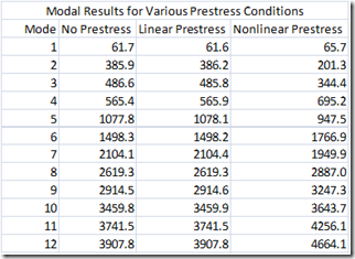
Here is a table of frequency results for a simple test case. Three modal analyses were run:
1. No prestress at all.
2. With a linear static prestress state.
3. With a nonlinear static prestress state.
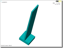
Here is the model used for these runs in its initial configuration. The block at the base was fixed in all DOF’s and the preload applied was a pressure load on one side of the vane.
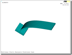
Here is the model with the deformed mesh due to the nonlinear prestress:
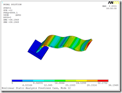
Here is a mode shape plot for mode 12:
The above example is all well and good but could have been done in prior versions of ANSYS using the old partial solve method. What’s nice about the newer linear perturbation method is that it’s easy to get the mode shape plots relative to the deformed mesh from the prior prestress run, and you don’t need to worry about over-writing the prestress results with the modal results, since the corresponding results files are different.
Further, we can now perform modal analyses using different restart points in the static prestress run, assuming multiple restart points are available.
Finally, we can actually change some contact options between the static prestress solution and the modal solution. For example, if the prestress analysis was run using frictional contact, the subsequent modal analysis can be run utilizing the prestressed state of the structure but with one of three contact states for the modal analysis: true status (that of the prior static analysis), force (to be) sticking, or force (to be) bonded. The sticking option applies only to contact elements with a nonzero coefficient of friction. The bonded option will force contact pairs that are in contact in the static analysis to be bonded in the modal analysis.
The Mechanical APDL command sequence for this procedure would be something like this:
! first perform nonlinear static prestress run, then
/solu
antype,,restart,,,perturbation
perturb,modal,,BONDED,PARDELE ! pre-stress modal analysis, switch contact to bonded, delete
! loads in case future MSUP
solve ! Generate matrices needed for perturbation analysis
! Next perform modal analysis
modopt,lanb,6
mxpand ! default expand in case of complex solution
solve
! modal results are now available for postprocessing
In Workbench Mechanical, the appropriate command sequence is sent to the solver when we link a modal analysis to a prior prestress analysis. If the model involves contact, then in the modal analysis we’ll have choices for how the contact should be treated in the Pre-Stress branch under the Modal branch in the Outline Tree. For frictional contact in the static prestress analysis, the choices in the Details view for the Pre-Stress branch in the modal analysis will be Use True Stress, Force Sticking, or Force Bonded as described above.
Here are some example plots for this scenario:
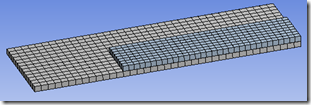
Two 3D plates subject to in plane bending, fixed at right ends, frictional contact between them.
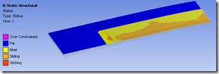
Resulting contact status for static run (sliding is occurring)
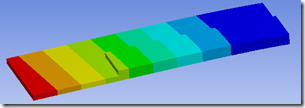
Resulting static deformation:
Mode 6 result, “true” contact behavior:
Mode 6 result, “force bonded” contact behavior:
Those last two images show a dramatic difference in modal results simply by changing the contact status behavior in the modal analysis. In the first of those images, the contact status is set to ‘true’, meaning essentially the same as in the prestress analysis, subject to the linear nature of the modal analysis. In this example, the frictional behavior in the static prestress run becomes no separation in the modal analysis, so the two plates can have mode shapes in which the plates slide relative to each other. In the last plot, the contact status has been changed to ‘force bonded’ for the modal solution. As the plot shows, mode shapes can only exist in which the two plates are bonded together. Both modal analyses have the same prestress condition however.
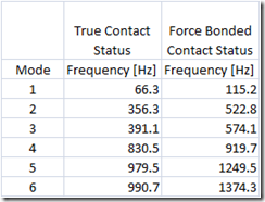
Here is a frequency table comparing the first six modes of the two modal analyses. Note that with the contact forced to be bonded we get a stiffening response as we might expect.
So, although on the surface it might initially appear to be a black art, linear perturbation is a nice enhancement in ANSYS 13.0 that gives us a more robust and capable method for performing modal analyses with prestress effects included. The prestress run is typically a linear or nonlinear static analysis, but it will also work with a full transient analysis to define the prestress state. The ANSYS 13.0 Help has more information (see section 9.2 of the Mechanical APDL Structural Analysis Guide and section 17.8 of the Theory Reference). We also recommend you try out the procedure on your own models.

