APDL Math. It is one of the most powerful, uber-user, deep down under the hood, wrapping your hands around the neck of what FEA is, capabilities in the ANSYS Mechanical APDL (MAPDL) solver. And most users don’t even know it is there. It kind of snuck in over time, with the developers adding more and more capability each release. Now it gives you access that you needed custom FORTRAN code to get to in the past… or NASTRAN DMAP, which is really something none of us ever want to do.
There is a lot of capability in this tool. This posting is just going to cover the basics so that you know what the tool can be used for in case you need it in the future, and hopefully motivate some of you to take a long look at the help.
What is APDL Math?
It is an extension to the APDL command language that drives MAPDL. Although it runs in a different workspace (chunk of memory in the ANSYS database) it talks to standard APDL by importing and exporting APLD arrays (vectors or matrices). It consists, at R14, of 18 commands that can be executed at the /SOLU level at any time. All of the commands start with a * character and look and act like standard APDL commands.
APDL Math is a tool for users to do two things: 1) get access to view, export or modify matrices and vectors created by the solver, and 2) to control import or modify matrices and vectors then solve them. The most common uses we have seen is the exporting of a matrix from ANSYS for use in some other program, usually Matlab. The other is working with sub-structure matrices.
The entire tool is documented in the Mechanical APDL section of the help under // ANSYS Parametric Design Language Guide // 4. APDL Math.
The Commands
Below is a list of the APDL math commands. As usual, you really need to read the manual entries to get the full functionality explained. Just like parameters and arrays in APDL, the matrices and vectors in APDL Math use names to identify them. Note that you have a set of commands to create the matrix/vector you want, which includes reading from a file or importing an APDL array. then you have commands to do basic matrix/vector math like multiply, find dot products, and do Fast Fourier Transformations. Then there are solver commands.
| Commands to create and delete matrices and vectors |
| *DMAT, Matrix, Type, Method, Val1, Val2, Val3, Val4, Val5 |
| Creates a dense matrix that is complex, double or integer. You can allocate it, resize an existing matrix, copy a matrix, or link to a portion of a matrix. You can also import from a file or an APDL variable. |
| *SMAT, Matrix, Type, Method, Val1, Val2, Val3 |
| Creates a sparse matrix. Double or Complex, copied or imported. |
| *VEC, Vector, Type, Method, Val1, Val2, Val3, Val4 |
| Creates a vector. Double, complex or integer. Similar arguments to *DMAT. |
| *FREE, Name, |
| Deletes a matrix or a solver object and frees its memory allocation. Important to remember to do. |
| Commands to manipulate matrices |
| *AXPY, vr, vi, M1, wr, wi, M2 |
| Performs the matrix operation M2= v*M1 + w*M2. |
| *DOT, Vector1, Vector2, Par_Real, Par_Imag |
| Computes the dot (or inner) product of two vectors. |
| *FFT, Type, InputData, OutputData, DIM1, DIM2, ResultFormat |
| Computes the fast Fourier transformation of the specified matrix or vector. |
| *INIT, Name, Method, Val1, Val2, Val3 |
| Initializes a vector or dense matrix. Used to fill vectors or matrices with zero’s, constant values, random values, or values on the diaganol. |
| *MULT, M1, T1, M2, T2, M3 |
| Performs the matrix multiplication M3 = M1(T1)*M2(T2). |
| *NRM, Name, NormType, ParR, Normalize |
| Computes the norm of the specified vector or matrix. |
| *COMP, Matrix, Algorithm, Threshold |
| Compresses the columns of a matrix using a specified Singular value decomposition algorithm (default) or Modified Gram-Schmidt algorithm |
| Commands to perform solutions |
| *LSENGINE, Type, EngineName, Matrix, Option |
| Creates a linear solver engine and assignes a name to be used when you want to execute the solve. Does Boeing sparse, MKL sparse, LAPACK or Distributed Sparse. |
| *LSFACTOR, EngineName, Option |
| Performs the numerical factorization of a linear solver system. |
| *LSBAC, EngineName, RhsVector, SolVector |
| Performs the solve (forward/backward substitution) of a factorized linear system. |
| *ITENGINE, Type, EngineName, PrecondName, Matrix, RhsVector, SolVector, MaxIter, Toler |
| Performs a solution using an iterative solver. |
| *EIGEN, Kmatrix, Mmatrix, Cmatrix, Evals, Evects |
| Performs a modal solution with unsymmetric or damping matrices. |
| Commands to output matrices |
| *EXPORT, Matrix, Format, Fname, Val1, Val2, Val3 |
| Exports a matrix to a file in the specified format. Supports Matrix Market, ANSYS SUB, DMIG, Harwell-Boeing and ANSYS EMAT. Also used to put values in an APDL array or print in a formated way to a postscript file. |
| *PRINT, Matrix, Fname |
| Prints the non-zero matrix values to a text file. |
| Useful APDL Commands |
| /CLEAR, Read |
| Wipes all APDL and APDL Math values from memory |
| WRFULL, Ldstep |
| Stops solution after assembling global matrices. Use this to make matrices you need when you don’t want a full solve |
| /SYS, String |
| Executes an operating system command. This can be used in APDL Math to do some sort of an external operation on a matrix you wrote out to a file, like running a matlab script. After execution the matrix can be read back in and used. |
How You Use APDL Math
When using APDL math you should follow some basic steps. I’m always a big proponent of the crawl-walk-run approach to anything, so I also recommend that you start with small, simple models to figure stuff out.
First Step: Know the Math
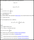 The first step, or maybe the zero’th, is to understand your math. If you charge in and start grabbing the stiffness matrix from the .FULL file and changing values, who knows what you will end up with. Chart out the math you want to do on paper or in a tool like Mathematica.
Then makes sure that you understand the math in ANSYS, and that includes the files being used by ANSYS. A good place to look is in the Programmer’s Manual, Chapter 1 lists the various files and what is in them. It might also not be a bad idea for you to crack open the theory manual We all know that ANSYS solve Kx = F, but how, and what matrices and vectors are used. Section 17.1 explains the static analysis approach used, with lots of links to more detailed explanations.
Second Step: Create your Matrices/Vectors
Since the whole point of using APDL math is to do stuff with Matrices/Vectors, you need to start by creating them. Note that we are not doing anything with APDL Math yet. We are using APDL, ANSYS, or an external program to get our matrix/vector so that we can then get it into APDL Math.. There are three types of sources you can get matrices/vectors from:
- Use APDL to create an array. *DIM, *SET, *VREAD, *MOPER, etc…
- Use ANSYS to make them as part of a solve, or as part of an “almost solve” using WRFULL. You can read the .FULL, .EMAT, .SUB, .MODE or .RST
- Get a file from some other source and put it into a format that APDL Math can read. It supports Harwell-Boeing, Matrix Market, or NASTRAN DMIG format as well as APDL Math’s own format.
Third Step: Get the Matrices/Vectors into APDL Math
Using *DMAT, *SMAT, and *VEC you convert the APDL array, ANSYS file, or external format file into a matrix or a vector. You can also use *INIT to make one from scratch, filling it with constants, zeros, random numbers or by setting the diagonal or anti-diagonal values.
Fourth Step: Manipulate the Matrices/Vectors
In this step you can modify matrices in a lot of different ways. The simplest is to use *MULT or *AXPY to do math with several matrices/vectors to get a new matrix/vector.
Another simple way to change things is to simply refer to the entries in the matrix using APDL. As an example, to change the damping at I=4 and J =5 in a damping matrix called dmpmtrx just use dmpmtrx(4,5) – 124.321e4.
You can take that one step further and use the APDL operators that work on arrays like *SET, *MOPER, *VGUN and whatever *DO loops you need.
If you can’t do the modification you need in APDL or APDL Math, then you can use *EXPORT to write the matrices out and use an external tool like matlab or Mathematica to do your manipulation. Of course you then use *DMAT with an IMPORT argument to read the modified matrix/vector back inside.
Fifth Step: Use the Matrix
Now it is finally time to use your matrices/vectors. The most common use is to bundle it up in a substructure matrix (*EXPORT,,SUB) and use it in a solve. What is great about this is that you can also (I know, we don’t want to use the N-word) save the file as a NASTRAN substructure and give it to that annoying DMAP guru who insists that NASTRAN is the only structural analysis code in the world. He gets his file, and you get to use ANSYS.
You can also solve using APDL Math. This can require multiple steps depending on what you want to do. A typical solve involves using the *LSENGINE command to define how you want to solve, then factor your matrix with *LSFACTOR, then solve with *LSBAK.
There are also ways to continue a solve in ANSYS after changing the EMAT file. Unfortunately my plans to do an example of this have been thwarted and ANSYS did not provide one, so I’m not 100% sure on the steps required. But a LSSOLVE that does not force ANSYS to recreate the matrices should work. Maybe a topic for a future posting.
Other Stuff to Know About
There is a lot more too this, and the help is where you can learn more. But a few things everyone needs to be ware of are listed here.
DOF Order
A key area where people have problems is understanding how the DOF’s in your matrix or vector are ordered. This is because ANSYS reorders things for efficiency of memory and solve. The nice thing is that ANSYS stores a map in the full file that you can use to convert back and forth using the *MULT command.
Please read section 4.4 ( // ANSYS Parametric Design Language Guide // 4. APDL Math // 4.4. Degree of Freedom Ordering) in the manual. They have a great description and some examples.
Just remember to remember to deal with DOF ordering.
Limitations
This is still a new tool set and as users apply it to real world problems, they are adding functionality. Right now there are some limitations.
- The biggest is that that all of this works on linear matrices. So you have to be working on a linear problem. Material or geometric non-linarites just don’t work. This makes perfect sense but may be one of those things some users might not figure out till they have invested some serious time.
- You can not modify a sparse matrix in APDL Math. You have to write it out using *EXPORT, modify it with something like matlab, then read it back in with *SMAT.
- *MULT can not be used to multiply two sparse matrices. One or both must be dense. the result is always dense.
- The BCS, DSS and DSP solves only work with sparse matrices. Only the LAPACK solver works for a dense matrix.
 Real and Imaginary
Most of the features in APDL math work with matrices that have imaginary terms in them. Be careful and read the help if you are using complex math, it can get tricky. Especially read 4.3 on how to specify a position in a matrix for real or imaginary numbers.
Examples
There are not a lot out there. The manual has some in section 4.7. Take a look at these before you do anything. If you can not find a specific example, contact your technical support provider and see if they have one, or if they can ask development for one.
Give it a Shot, and Share
This is a new feature, and a power user feature. So what is happening is some very smart people are doing some very cool things with it, and not sharing. It is very important that you share your effort with your Channel Partner or ANSYS, Inc so that they can not only see how people use this tool, but also modify the tool to do even more cool things.
It would also be cool if you posted what you do on XANSYS for the masses to see. Very cool.


