
Postprocessing results along a path has been part of the Workbench Mechanical capability for several rev’s now. We need to define a path as construction geometry on which to map the results unless we happen to have an edge in the model exactly where we want the path to be or can use an X axis intersection with our model. You have the option to ‘snap’ the path results to nodal locations, but what if you want to use nodal locations to define the path in the first place? We’ll see how to do this below.
For more information on “picking your nodes”, see the Focus blog entry written by Jeff Strain last year: https://www.padtinc.com/blog/the-focus/node-interaction-in-mechanical-part-1-picking-your-nodes
The top level process for postprocessing result along a path is:
- Define a Path as construction geometry
- Insert a Linearized Stress result
- Calculate the desired results along the path using the Linearized Stress item
The key here is to define the path using existing nodes. Why do that? Sometimes it’s easier to figure out where the path should start and stop using nodal locations rather than figure out the coordinates some other way. So, let’s see how we might do that.
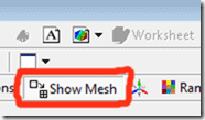
- First, turn on the mesh via the “Show Mesh” button so that it’s visible for the path creation

- From the Model branch in Mechanical, insert Construction Geometry
- From the new Construction Geometry branch, insert a Path

- Note that the Path must be totally contained by the finite element model, unlike in MAPDL.
- If you know the starting and ending points of the path, enter them in the Start and End fields in the Details view for the Path.
- Otherwise, click on the “Hit Point Coordinate” button:

- Pick the node location for the start point, click apply

- Pick the node location for the end point, click apply

- In the Solution branch, insert Linearized Stress (Normal Stress in this case); set the details:
- Scoping method=Path
- Select the Path just created
- Set the Orientation and Coordinate System values as needed
- Define Time value for results if needed

Results are displayed graphically along the path…

…as well is in an X-Y plot and a table

Besides normal stresses, membrane and bending, etc. results can be accessed using these techniques. So, the next time you need to list or plot results along a path, remember that it can be done in Mechanical, and you can use nodal locations to define the starting and ending points of the path.


