Editors Note (2/2/2023): We originally uploaded this ACT extension to the Ansys Store, but have since decided to keep the updated versions here on the PADT blog. You can read about the latest update in “Ansys ACT Extension for a PID Thermostat Controller – Updated, February 2023.“ You can also download the latest version in that post.
I’m going to embark on a multipart blog series chronicling my efforts in writing a PID Thermostat control boundary condition for workbench. I picked this boundary condition for a few of reasons:
- As far as I know, it doesn’t exist in WB proper.
- It involves some techniques and element types in ANSYS Mechanical APDL that are not immediately intuitive to most users. Namely, we will be using the Combin37 element type to manage the control.
- There are a number of different options and parameters that will be used to populate the boundary condition with data, and this affords an opportunity to explore many of the GUI items exposed in ACT.
This first posting goes over how to model a PID controller in ANSYS Mechanical APDL. In future articles I will share my efforts to refine the model and us ACT to include it in ANSYS Workbench.
PID Controller Background
Let’s begin with a little background on PID controllers. Full disclaimer, I’m not controls engineer, so take this info for what it is worth. PID stands for Proportional Integral Differential controller. The idea is fairly simple. Assume you have some output quantity you wish to control by varying some input value. That is, you have a known curve in time that represents what you would like the output to look like. For example:
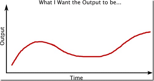
The trick is to figure out what the input needs to look like in time so that you get the desired output. One way to do that is to use feedback. That is, you measure the current output value at some time, t, and you compare that to what the desired output should be at that time, t. If there is no difference in the measured value and the desired value, then you know whatever you have set the input to be, it is correct at least for this point in time. So, maybe it will be correct for the next moment in time. Let’s all hope…
However, chances are, there is some difference between what is measured and what is desired. For future reference we will call this the error term. The secret sauce is what to do with that information? To make things more concrete, we will ground our discussion in the thermal world and imagine we are trying to maintain something at a prescribed temperature. When the actual temperature of the device is lower than the desired temperature, we will define that as a positive error. Thus, I’m cold; I want to be warmer: that equals positive error. The converse is true. I’m hot; I want to be colder: that equals negative error.
One simple way we could try to control the input would be to say, “Let’s make the input proportional to the error term.” So, when the error term is positive, and thus I’m cold and wish to be warmer, we will add energy proportionate to the magnitude of the error term. Obviously the flip side is also true. If I’m hot and I wish to be cooler my negative error term would mean that remove energy proportionate to the magnitude of the error term. This sounds great! What more do you need? Well, what happens if I’m trying to hold a fixed temperature for a long time? If the system is not perfectly adiabatic, we still have to supply some energy to make up for whatever the system is losing to the surroundings. Obviously, this energy loss occurs even with the system is in a steady state configuration and at the prescribed temperature! But, if the system is exactly at the prescribed temperature, then the error term is zero. Anything proportionate to zero is… zero. That’s a bummer. I need something that won’t go to zero when my error term goes to zero.
What if I could keep a record of what I’ve done in the past? What if I accumulated all of the past error from forever? Obviously, this has the chance of being nonzero even if instantaneously my error term is zero. This sounds promising. Integrating a function of time with respect to time is analogous to accumulating the function values from history past. Thus, what if I integrated my error term and then made my input also proportional to that value? Wouldn’t that help the steady state issue above? Sure it would. Unfortunately, it also means I might go racing right on by my set point and it might take a while for that “mistake” to wash out of the system. Nothing is free. So, now I have kept a record of my entire past and used that to help me in the present, what if I could read the future? What if could extrapolate out in time?
Derivatives allow us to make a local extrapolation (in either direction) about a curve at a fixed point. So, if my curve is a function of time, which in our case the curves are, forward extrapolation is basically jumping ahead into the future. However, we can’t truly predict the future, we can only extrapolate on what has recently happened and make the leap of faith that it will continue to happen just as it has. So, if I take the derivative of my error term with respect to time, I can roll the dice a little a make some of my input proportional to this derivative term. That is, I can extrapolate out in time. If I do it right, I can actually make the system settle out a little faster. Remember that when the error term goes to zero and stays there, the derivative of the error term also goes to zero. So, when we are right on top of our prescribed value this term has no bearing on our input.
So, a PID controller simply takes the three concepts of how to specify an input value based on a function of the error term and mixes them together with differing proportions to arrive at the new value for the input. By “tuning” the system we can make it such that it responds quickly to change and it doesn’t wildly overshoot or oscillate.
Implementing a PID controller in ANSYS MAPDL
We will begin by implementing a PID controller in MAPDL before moving on to implementing the boundary condition in ANSYS Workbench via the ACT. We would like the boundary condition to have the following features:
- Ultimately we would like to “connect” this boundary condition to any number of nodes in our model. That is, we may want to have our energy input occur on a vertex, edge or face of the model in Workbench. So, we would like the boundary condition to support connecting to any number of nodes in the model.
- Likewise, we would like the “measured output” to be influenced by any number of nodes in our model. That is, if more than one node is included in the “measured value” set, we would like ANSYS to use the average temperature of the nodes in that set as our “measured output”. Again, this will allow us to specify a vertex, edge, face or body of the model to function as our measurement location. The measured value should be the average temperature on this entity. Averaging needs to be intelligent. We need to weight the average based on some measure that accounts for the relative influence of a node attached to large elements vs one attached to small elements.
- We would like to be able to independently control the proportional, integral and derivative components of the control algorithm.
- It would be nice to be able to specify whether this boundary condition can only add energy, only remove energy or if it can do both.
- We would like to allow the set point value to also be a function of time so that it too can change with time.
- Finally, it would be nice to be able to post process some of the heat flow quantities, temperature values, etc… associated with this boundary condition.
This is a pretty exhaustive list of requirements for the boundary condition. Fortunately, ANSYS MAPDL has built into it an element type that is perfectly suited for this type of control. That element type is the combin37.
Introducing the Combin37 Element Type
Understanding the combin37 element in ANSYS MAPDL takes a bit of a Zen state of mind… It’s, well, an element only a mother could love. Here is a picture lifted from the help:
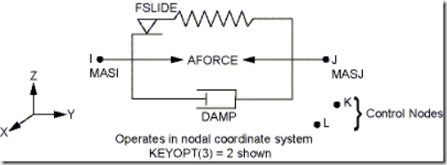
OK. Clear as mud right? Actually, this thing can act as a thermostat whether you believe me from the picture or not. Like most/all ANSYS elements that can function in multiple roles, the combin37 is expressed in its structural configuration. It is up to you and me to mentally map it to a different set of physics. So, just trust me that you can forget the damping and FSLIDE and little springy looking thing in the picture. All we are going to worry about is the AFORCE thing. Mentally replace AFORCE with heat flow.
Notice those two little nodes hanging out there all by their lonesome selves labeled “control nodes”. I think they should have joysticks beside them personally, but ANSYS didn’t ask me. Those little guys are appropriately named. One of them, NODE K actually, will function as our set point node. That is, whatever temperature value we specify in time for NODE K, that same value represents the set point temperature we would like our “measured” location take on in time as well. So, that means we need to drive NODE K with our set point curve. That should be easy enough. Just apply a temperature boundary condition that is a function of time to that node and we’re good to go. Likewise, NODE L represents the “measured” temperature somewhere else in the model. So, we need to somehow hook NODE L up to our set of measurement nodes so that it magically takes on the average value of those nodes. More on that trick later.
Now, internally the combin37 subtracts the temperature at NODE K from NODE L to obtain an error term. Moreover, it allows us to specify different mathematical operations we can perform on the error term, and it allows us to take the output from those mathematical operations and drive the magical AFORCE thingy, which is heat flow. Guess what those mathematical operations are? If you guessed simply making the heat flow through the element proportional to the error, proportional to the time integral of the error and proportional to the time derivative of the error you would be right. Sounds like a PID controller doesn’t it? Now, the hard part is making sense of all the options and hooking it all up correctly. Let’s focus on the options first.
Key Option One and the Magic Control Value
Key option 1 for the combin37 controls what mathematical operation we are going to perform on the error term. In order to implement a full PID controller, we are going to need three combin37 elements in our model with each one keyed to a different mathematical operation. ANSYS calls the result of the mathematical operation, Cpar. So, we have the following:
| KEYOPT(1) Value | Mathematical Operation |
| 0,1 | |
| 2 | |
| 3 | |
| 4 | |
| 5 |
Thus, for our purposes, we need to set keyopt(1) equal to 1,4 and 2 for each of the three elements respectively.
Feedback is realized by taking the control parameter Cpar and using it to modify the heat flow through the element, which is called AFORCE. The AFORCE value is specified as a real constant for the element; however, you can also rig up the element so that the value of AFORCE changes with respect to the control parameter. You do this by setting keyopt(6)=6. The manner in which ANSYS adjusts the AFORCE value, which again is heat flow, is described by the following equation:

Thus, the proportionality constant for the Proportional, Integral and Derivative components are specified with the C1 variable. RCONST, C3 and C4 are all set to zero. C2 is set to 1. Also note that ANSYS first takes the absolute value of the control parameter Cpar before plugging it into this equation. Furthermore, the direction of the AFORCE component is important. A positive value for AFORCE means that the element generates an element force (heatflow) in the direction specified in the diagram. That is, it acts as a heat sink. So, assuming the model is attached to node J, the element acts as a heat sink when AFORCE is positive. Conversely, when AFORCE is negative, the element acts like a heat source. However, due to the absolute value, Cpar can never take on a negative value. Thus, when this element needs to act as an energy source to add heat to our model, the coefficient C1 must be negative. The opposite is true when the element needs to act as an energy sink.
Key Option Four and Five and when is it Alive?
If things weren’t confusing enough already, hold on as we discuss Keyopt 4 and 5. Consider the figure below, again lifted straight from the help.
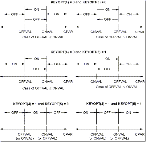
The combination of these two key options controls when the element switches on and becomes “alive”. Let’s take the simple case first. Let’s assume that we are adding energy to the model in order to bring it up to a given temperature. In this case, Cpar will be positive because our set point is higher than our current value. If the element is functioning as a heat source we would like it to be on in this condition. Furthermore, we would like it to stay on as long as our error is positive so that we continue adding energy to bring the system up to temperature. Consider the diagram in the upper left. Imagine that we set ONVAL = 0 and OFFVAL = 0.001. Whenever Cpar is greater than ONVAL. So this sounds like exactly what we want when the element is functioning as a heat source. Thus, keyopt(4)=0 and keyopt(5)=0.001 with OFFVAL=ONVAL=0 is what we want when the element needs to function as a heat source.
What about when it is a heat sink? In this case we want the element to be active when the error term is negative; that is, when the current temperature is higher than the set point temperature. Consider the diagram in the middle left. This time let OFFVAL=0 and OFFVAL=-0.001. In this case, whenever Cpar is negative (less than OFFVAL) then the element will be active. Thus, keyopt(4)=0 and keyopt(5)=1 with OFFVAL=-0.001 ONVAL=0 is what we want when the element needs to function as a heat sink. Notice, that if you set ONVAL=OFFVAL then the element will always stay on; thus, we need to provide the small window to activate the switching nature of the element.
Thus, we see that we need six different combin37 elements, three for a PID controlled heat sink and three for a PID controlled heat source, to fully specify a PID controlled thermal boundary condition. Phew… However, if we set all of the proportionality constants for either set of elements defining the heat sink or heat source to zero, we can effectively turn the boundary condition into only a heat source or only a heat sink, thus meeting requirement four listed above. While we’re marking off requirements, we can also mark off requirements three and five. That is, with this combination of elements we can independently control the P, I and D proportionality constants for the controller. Likewise, by putting a time varying temperature constraint on control node K, we can effectively cause the set point value to change in time. Let’s see if we can now address requirements one and two.
How do we Hook the Combin37 to the Rest of the Model?
We will address this question in two parts. First, how do we hook the “business” end of the combin37 to the part of the model to which we are going to add or remove energy? Second, how do we hook the “control” end of the combin37 to the nodes we want to monitor?
Hooking to the Combin37 to the Nodes that Add or Remove Energy
To hook the combin37 to the model so that we can add or remove energy we will use the convection link elements, link34. These elements effectively act like little thermal resistors with the resistance equation being specified as:

In order to make things nice, we need to “match” the resistances so that each node effectively sees the same resistance back to the combin37 element. We do this by varying the “area” associated with each of these convective links. To get the area associated with a node we use the arnode() intrinsic function. See the listing for details.
Hooking the Combin37 to the Nodes that Function as the Measured Value
As we mentioned in our requirements, we would like to be able to specify more than one or more nodes to function as the measured control value for our boundary condition. More precisely, if more than one node is included in the measurement node set, we would like ANSYS to average the temperatures at those nodes and use that average value as the measurement temperature. This will allow us to specify, for example, the average temperature of a body as the measurement value, not just one node on the body somewhere. However, we would also like for the scheme to work seamlessly if only one node is specified. So, how can we accomplish this? Constraint equations come to our rescue.
Remember that a constraint equation is defined as:

How can we use this to compute the average temperature of a set of nodes, and tie the control node of the combin37 to this average? Let’s begin by formulating an equation for the average temperature of a set of nodes. We would like this average to not be simply a uniform average, but rather be weighted by the relative contribution a given node should play in the overall average of a geometric entity. For example, assume we are interested in calculating the average temperature of a surface in our model. Obviously this surface will have associated with it many nodes connected to many different elements. Assume for the moment that we are interested in one node on this face that is connected to many large elements that span most of the area of this face. Shouldn’t this node’s temperature have a larger contribution to the “average” temperature of the face as say a node connected to a few tiny elements? If we just add up the temperature values and divide by the number of nodes, each node’s temperature has equal weight in the average. A better solution would be to area weight the nodal temperatures based on the area associated with each individual node. Something like:

That looks a little like our constraint equation. However, in the constraint equation I have to specify the constant term, whereas in the equation above, that is the value (Tavg) that I am interested in computing. What can I do? Well, let’s add in another node to our constraint equation that represents the “answer”. For convenience, we’ll make this the control node on our combin37 elements since we need the average temperature of the face to be driving that node anyway. Consider:

Now, our constant term is zero, and our Ci’s are Ai/AT and -1 for the control node. Voila! With this one constraint equation we’ve compute an area weighted average of the temperature over a set of nodes and assigned that value to our control node. CE’s rock!
An Example Model
This post is already way too long, so let’s wrap things up with a little example model. This model will illustrate a simple PI heat source attached to an edge of a plate with a hole. The other outer edges of the plate are given a convective boundary condition to simulate removing heat. The initial condition of the plate is set to 20C. The set point for the thermostat is set to 100C. No attempt is made to tune the PI controller in this example, so you can clearly see the effects of the overshoot due to the integral component being large. However, you can also see how the average temperature eventually settles down to exactly the set point value. 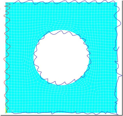
The red squiggly represents where heat is being added with the PI controller. The blue squiggly represents where heat is being removed due to convection. Here is a plot of the average temperature of the body with respect to time where you can see the response of the system to the PI control.
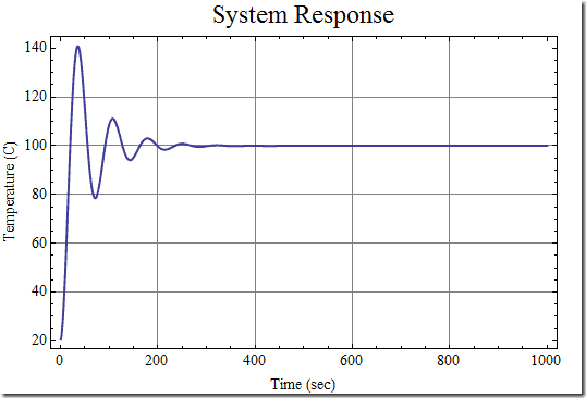
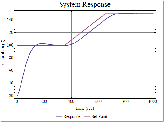
Here is another run, where the set point value ramps up as well. I’ve also tweaked the control values a little to mitigate some of the overshoot. This is looking kind of promising, and it is fun to play with. Next time we will look to integrate it into the workbench environment via an actual ACT extension.
Part 2 is here
Model Listing
I’ve included the model listing below so that you can play with this yourself. In future posts, I will elaborate more on this technique and also look to integrate it into an ACT module.
finish
/clear

/prep7
*get,etmax_,etyp,0,num,max
P_et=etmax_+1
I_et=etmax_+2
D_et=etmax_+3
Link_et=etmax_+4
mass_et=etmax_+5

et,P_et,combin37
et,I_et,combin37
et,D_et,combin37
et,Link_et,link34
et,mass_et,mass71
Kp=1
Ki=2
Kd=0

keyopt,P_et,1,0    ! Control on UK-UL
keyopt,P_et,2,8    ! Control node DOF is Temp
keyopt,P_et,3,8    ! Active node DOF is Temp
keyopt,P_et,4,0    ! Wierdness for the ON/OFF range
keyopt,P_et,5,0    ! More wierdness for the ON/OFF range
keyopt,P_et,6,6    ! Use the force, Luke (aka Combin37)
keyopt,P_et,9,0    ! Use the equation, Duke (where is Daisy...)


keyopt,I_et,1,4    ! Control on integral wrt time
keyopt,I_et,2,8    ! Control node DOF is Temp
keyopt,I_et,3,8    ! Active node DOF is Temp
keyopt,I_et,4,0    ! Wierdness for the ON/OFF range
keyopt,I_et,5,0    ! More wierdness for the ON/OFF range
keyopt,I_et,6,6    ! Use the force, Luke (aka Combin37)
keyopt,I_et,9,0    ! Use the equation, Duke (where is Daisy...)


keyopt,D_et,1,2    ! Control on first derivative wrt time
keyopt,D_et,2,8    ! Control node DOF is Temp
keyopt,D_et,3,8    ! Active node DOF is Temp
keyopt,D_et,4,0    ! Wierdness for the ON/OFF range
keyopt,D_et,5,0    ! More wierdness for the ON/OFF range
keyopt,D_et,6,6    ! Use the force, Luke (aka Combin37)
keyopt,D_et,9,0    ! Use the equation, Duke (where is Daisy...)

keyopt,mass_et,3,1 ! Interpret real constant as DENS*C*Volume


!!!!!!!!!!!!!!!!!!!!!!!!!!!!!!!!!!!!!!!!!!!!!!!!!!
!!        S M A L L   T E S T   M O D E L       !!
!!!!!!!!!!!!!!!!!!!!!!!!!!!!!!!!!!!!!!!!!!!!!!!!!!
test_et=etmax_+10
et,test_et,plane55

mp,kxx,test_et,70
mp,dens,test_et,8050
mp,c,test_et,0.4
! Thickness of plate
r,test_et,0.1

! Plane55 element
keyopt,test_et,3,3

! Make a block
k,1
k,2,1,0
k,3,1,1
k,4,0,1
a,1,2,3,4
! Make a hole
cyl4,0.5,0.5,0.25
! Punch a hole
asba,1,2

type,test_et
mat,test_et
real,test_et
esize,0.025
amesh,all

! create an nodal component for the
! 'attachment' location
lsel,s,loc,x,0
nsll,s,1
cm,pid_attach_n,node

! create a nodal component for the
! 'monitor' location
allsel,all
cm,pid_monitor_n,node

!!!!!!!!!!!!!!!!!!!!!!!!!!!!!!!!!!!!!!!!!!!!!!!!!!
!!        B E G I N   P I D   M O D E L         !!
!!!!!!!!!!!!!!!!!!!!!!!!!!!!!!!!!!!!!!!!!!!!!!!!!!

! Real constant and mat prop for the mass element
mp,qrate,mass_et,0 ! Zero heat generation rate for the element
r,mass_et,1e-10  ! Extremely small thermal capacitance

! Material properties for convection element
! make the convection "large"
mp,hf,Link_et,1e5

! Real constant for the combin37 elements
! that ack as heaters
on_val_=0
off_val_=1e-3
r,P_et,0,0,0,on_val_,off_val_,0
rmore,0,1,-Kp,1

r,I_et,0,0,0,on_val_,off_val_,0
rmore,0,1,-Ki,1

r,D_et,0,0,0,on_val_,off_val_,0
rmore,0,1,-Kd,1

! build the PID elements
*get,nmax_,node,0,num,max
BASE_NODE=nmax_+1
P_NODE_J=nmax_+2
I_NODE_J=nmax_+3
D_NODE_J=nmax_+4
NODE_K=nmax_+5
NODE_L=nmax_+6
! Create the nodes.  They can be all coincident
! as we will refer to them solely by their number.
! They will be located at the origin
*do,i_,1,6
    n,nmax_+i_
*enddo

! Put a thermal mass on the K and L nodes
! for each control element to give them
! thermal DOFs
type,mass_et
mat,mass_et
real,mass_et
e,NODE_K
e,NODE_L

! Proportional element
type,P_et
mat,P_et
real,P_et
e,BASE_NODE,P_NODE_J,NODE_K,NODE_L

! Integral element
type,I_et
mat,I_et
real,I_et
e,BASE_NODE,I_NODE_J,NODE_K,NODE_L

! Derivative Element
type,D_et
mat,D_et
real,D_et
e,BASE_NODE,D_NODE_J,NODE_K,NODE_L


! Ground the base node
d,BASE_NODE,temp,0

! Get a list of the attachment nodes
cmsel,s,pid_attach_n
*get,numnod_,node,0,count
attlist_=
*dim,attlist_,,numnod_
*vget,attlist_(1),node,0,nlist
*get,rmax_,rcon,0,num,max

! Hook the attachment nodes to the
! end of the control element with
! convection links
*do,i_,1,numnod_
    n1_=attlist_(i_)
    a1_=arnode(n1_)
    r1_=rmax_+i_
    r,r1_,a1_
    type,link_et
    mat,link_et
    real,r1_
    e,P_NODE_J,n1_
    e,I_NODE_J,n1_
    e,D_NODE_J,n1_
*enddo

! Hook up the monitor nodes
cmsel,s,pid_monitor_n
*get,numnod_,node,0,count
monlist_=
monarea_=
*dim,monlist_,,numnod_
*dim,monarea_,,numnod_
*vget,monlist_(1),node,0,nlist
! We are going to need these areas
! so, hold on to them
*do,i_,1,numnod_
    monarea_(i_)=arnode(monlist_(i_))
*enddo
*vscfun,totarea_,sum,monarea_(1)
! Write the constraint equations
/pbc,ce,,0
ce,next,0,NODE_L,temp,-1
*do,i_,1,numnod_
    ce,high,0,monlist_(i_),temp,monarea_(i_)/totarea_
*enddo

! Create a transient setpoint temperature
*dim,setpoint_,table,2,,,time
setpoint_(1,0)=0
setpoint_(2,0)=3600
setpoint_(1,1)=100
setpoint_(2,1)=100

! Constrain the temperature node to be
! at the setpoint value
allsel,all
d,NODE_K,temp,%setpoint_%


! Apply an initial condition of
! 20 C to everything
allsel,all
ic,all,temp,20

/solu
antype,trans,new
time,1000
deltim,1,1,1
lsel,s,loc,x,0.1,1
nsll,s,1
sf,all,conv,20,20

allsel,all
outres,all,all
solve
/post26
! Plot the response temperature
! and the setpoint temperature
nsol,2,NODE_L,temp,,temp_r
nsol,3,NODE_K,temp,,temp_s
xvar,1
plvar,2,3


