If you've been following The Focus for a long time, you may recall my prior article about submodeling using ANSYS Mechanical APDL, which was a 'sub' model of a submarine. The article, from 2006, begins on page 2 at this link:
Also, Eric Miller here at PADT wrote a Focus blog entry on the new-at-14.5 submodeling capability in ANSYS Workbench Mechanical.
Since both of those articles were about structural submodeling, I decided it was time we published a blog entry on how to perform submodeling in ANSYS Mechanical for thermal simulations.
Submodeling is a technique whereby we can obtain more accurate results in a small, detailed portion of a large model without having to build an incredibly refined and detailed finite element model of our complete system. In short, we map boundary conditions onto a 'chunk' of interest that is a subset of our full model so that we can solve that 'chunk' in more detail. Typically we mesh the 'chunk' with a much finer mesh than was used in the original model, and sometimes we add more detail such as geometric features that didn't exist in the original model like fillets.
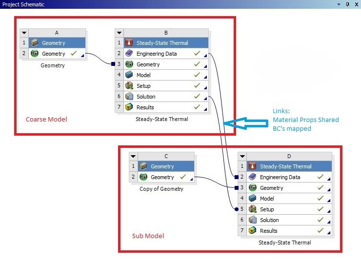
The ANSYS Workbench Project Schematic for a thermal solution involving submodeling looks like this:
Figure 1 – Thermal Submodeling Project Schematic
Note that in the project schematic, the links are automatically established when we setup the submodel after completing the analysis on the coarse model as we shall see below.
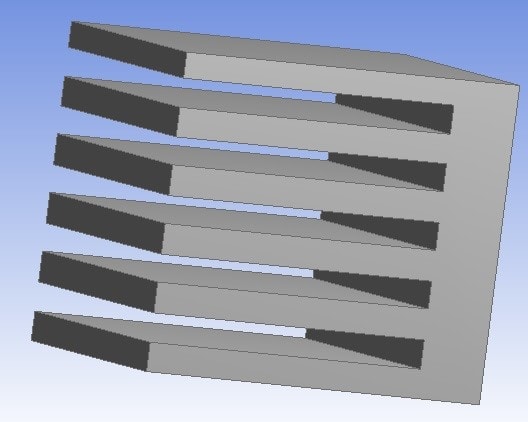
First, here is the geometry of the coarse model. It's a simple set of cooling fins. In this idealized model, no fillets have been modeled between the fins and the block.
Figure 2 – Coarse Model Geometry, Idealized without Fillets
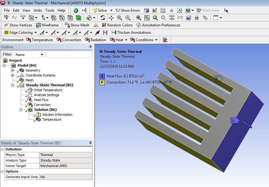
The boundary conditions consisted of a heat flux due to a thermal source on the base face and convection to ambient air on the cooling fin surfaces. The heat flux was setup to vary over the course of 3 load steps as follows:
Load Step Heat Flux (BTU/s*in^2)
1 0.2
2 0.5
3 0.005
Thus, the maximum heat going into the system occurs in load step 2, corresponding to 'time' 2.0 in this steady state analysis.
Figure 3 – Coarse Model Boundary Conditions – Heat Flux and Convection
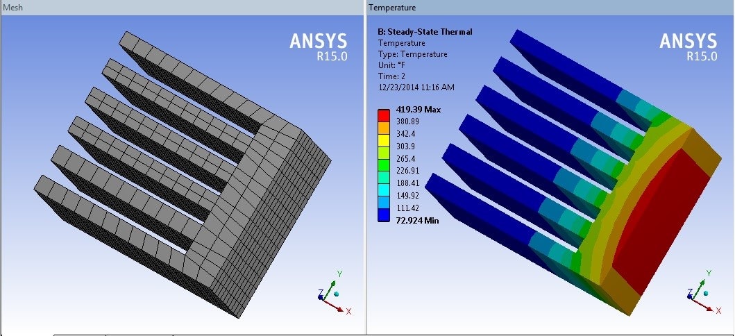
The coarse model is meshed with relatively large elements in this case. The mesh refinement for a production model should be sufficient to adequately capture the fields of interest in the locations of interest. After solving, the temperature results show a max temperature at the base where the heat flux is applied, transitioning to the minimum temperature on the cooling fins where convection is removing heat.
Figure 4 – Coarse Model Mesh and Temperature Results for Load Step 2
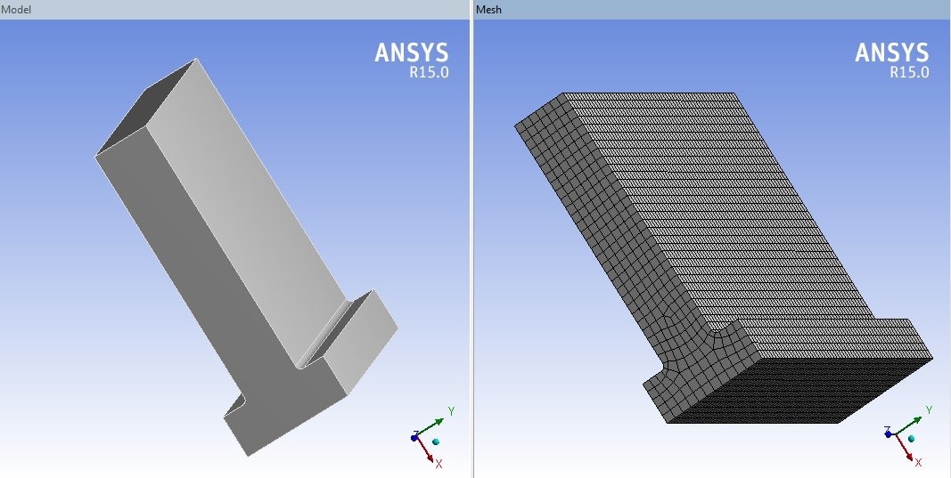
Our task now is to calculate the temperature in one of these fins with more accuracy. We will use a finer mesh and also add fillets between the fin and base. For this example, I isolated one fin in ANSYS DesignModeler, did some slicing, and added a fillet on either side of the base of the fin of interest.
Figure 5 – Fine Model (Submodel) Isolated Fin Geometry and Mesh, Including Fillets at Base
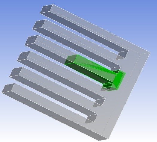
ANSYS requires that the submodel lie in the exact geometric position as it would in the coarse model, so it's a good idea to overlay our fine model geometry onto the coarse model to verify the positioning.
Figure 6 – Submodel and Coarse Model Overlaid
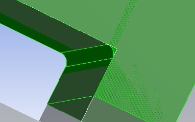
Figure 7 – Submodel and Coarse Model Overlaid, Showing Addition of Fillet
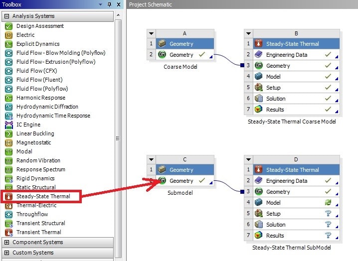
The next step is to insert the submodel geometry as a stand-alone geometry block in the Project Schematic which already contains the coarse model, as shown in figure 8. A new Steady-State Thermal analysis is then dragged and dropped onto the geometry block containing the submodel geometry.
Figure 8 – Submodel Geometry Added to Project Schematic, New Steady-State Thermal System Dragged and Dropped onto Submodel Geometry
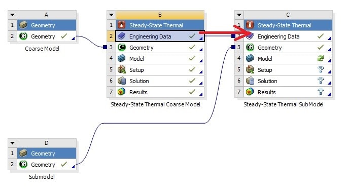
Next, we drag and drop the Engineering Data cell from the coarse model to the Engineering Data cell in the submodel block. This will establish a link so that the material properties will be shared.
Figure 9 – Drag and Drop Engineering Data from Coarse Model to Submodel
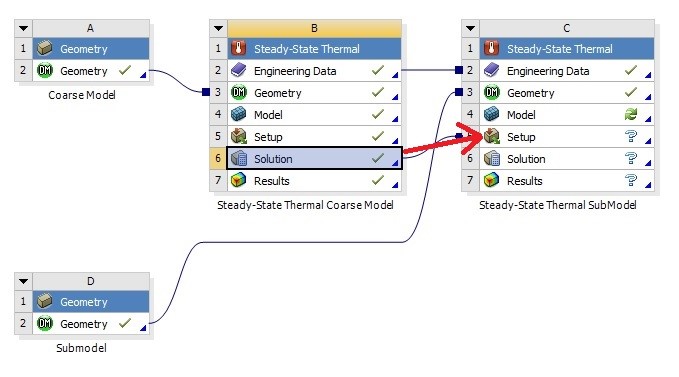
The final needed link is established by dragging and dropping the Solution cell from the coarse model onto the Setup cell in the submodel. This step causes ANSYS to recognize that we are performing submodeling, and in fact this will cause a Submodeling branch to appear in the outline tree in the Mechanical window for the submodel.
Figure 10 – Solution Cell Dragged and Dropped from Coarse Model to Submodel Setup Cell
After opening the Mechanical editor for the submodel block, we can see that the Submodeling branch has automatically been added to the tree.
Figure 11 – Submodeling Branch Automatically Added to Outline Tree
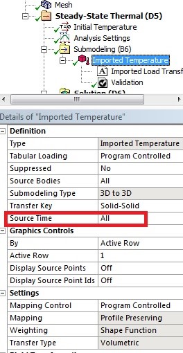
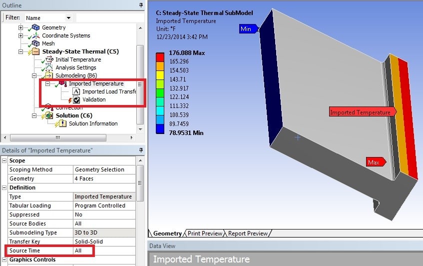
After meshing the submodel I specified that all three load steps should have their temperature data mapped to the submodel from the coarse model. This was done in the Details view for the Imported Temperature branch, by setting Source Time to All.
Figure 12 – Set Imported Temperature Source Time to All to Ensure All Loads Steps Are Mapped
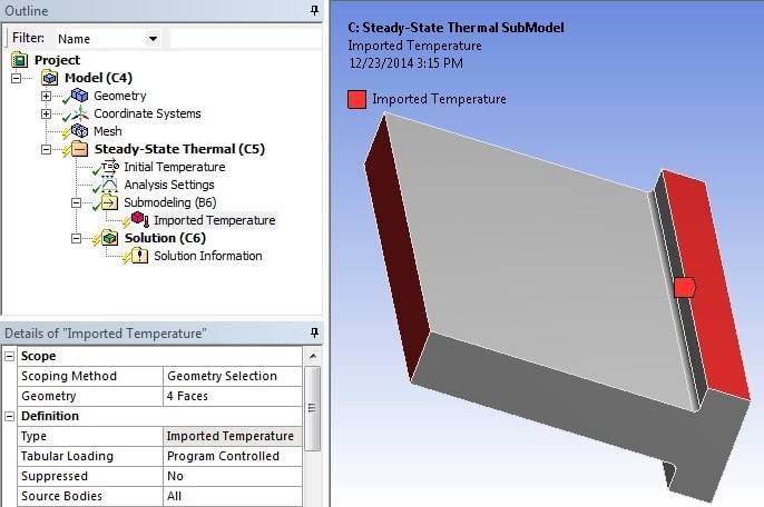
Next I selected the four faces that make up the cut boundaries in the submodel and applied those to the geometry selection for Imported Temperature.
Figure 13 – Cut Boundary Faces Selected for Imported Temperature
As mentioned above, the Imported Temperature details were set to read in all load steps by setting Source Time to All. The Imported Temperature branch can now be right-clicked and the resulting imported temperatures viewed. I also inserted a Validation branch which we will look at after solving.
Figure 14 – Setting Source Time to All, Viewing Imported Temperature on Submodel
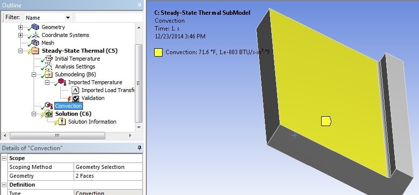
Any other loads that need to be applied to the submodel are added as well. For this model, it's convection on the large faces of the fin that are exposed to ambient air.
Figure 15 – Submodel Convection Load on Fin Exposed Faces
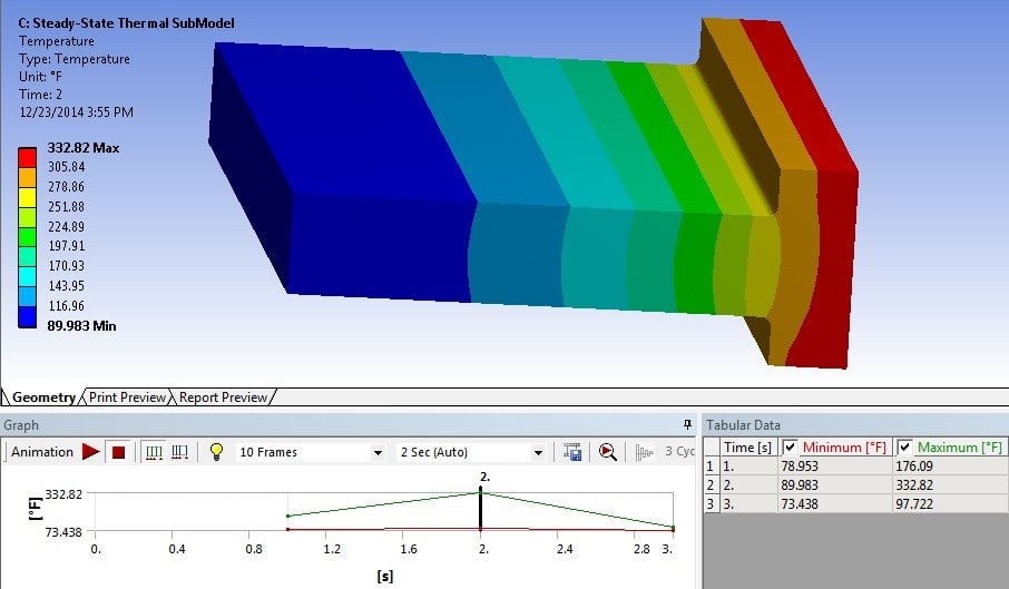
Since there are three load steps in the coarse model and we told ANSYS to map results from all time points, I set the number of steps to three in Analysis Settings, then solved the submodel. Results are available for all three load steps.
Figure 16 – Submodel Temperature Results for Step 2 (Highest Heat Flux Value in Coarse Model)
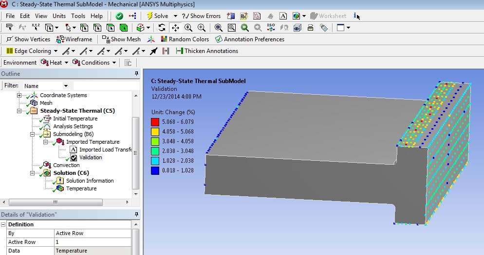
Regarding the Validation item under the Imported Temperature branch, this is probably best added after the solution is done. In my case I had to clear it and recalculate it. Validation can display either an absolute or relative (percent difference) plot on the nodes at which loads were imported. Figure 17 shows the relative difference plot, which maxes out at about 6%. The validation information as well as mapping techniques are described in the ANSYS Help.
Figure 17 – Submodel Imported Temperature Validation Plot – Percent Difference on Mapped Nodes
Looking at the coarse model and submodel results side by side, we see good agreement in the calculated temperatures. The temperature in the fillets shows a nice, smooth gradient.
Figure 18 – Coarse and Submodel Temperature Results Showing Good Agreement
Hopefully this explanation will be helpful to you if you have a need to perform submodeling in a thermal simulation in ANSYS. There is a Thermal Submodeling Workflow section in the ANSYS 15.0 Help in the Mechanical User's Guide that you may find helpful as well.


