HFSS offers various methods to define array excitations. For a large array, you may take advantage of an option “Load from File” to load the magnitude and phase of each port. However, in many situations you may have specific cases of array excitation. For example, changing amplitude tapering or the phase variations that happens due to frequency change. In this blog we will look at using the “Edit Sources” method to change the magnitude and phase of each excitation. There are cases that might not be easily automated using a parametric sweep. If the array is relatively small and there are not many individual cases to examine you may set up the cases using “array parameters” and “nested-if”.

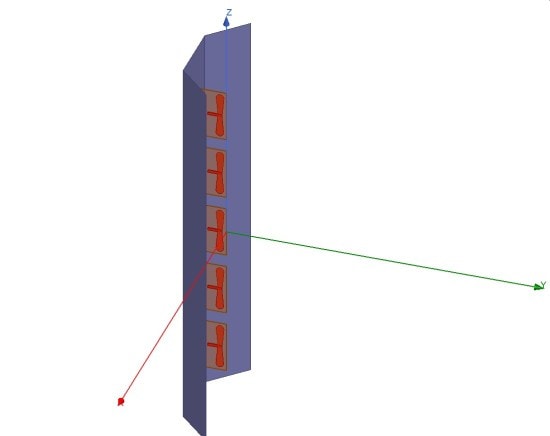
In the following example, I used nested-if statements to parameterize the excitations of the pre-built example “planar_flare_dipole_array”, which can be found by choosing File->Open Examples->HFSS->Antennas (Fig. 1) so you can follow along. The file was then saved as “planar_flare_dipole_array_if”. Then one project was copied to create two examples (Phase Variations, Amplitude Variations).

Fig. 1. Planar_flare_dipole_array with 5 antenna elements (HFSS pre-built example).

Phase Variation for Selected Frequencies

In this example, I assumed there were three different frequencies that each had a set of coefficients for the phase shift. Therefore, three array parameters were created. Each array parameter has 5 elements, because the array has 5 excitations:

A1: [0, 0, 0, 0, 0]

A2: [0, 1, 2, 3, 4]

A3: [0, 2, 4, 6, 8]

Then 5 coefficients were created using a nested_if statement. “Freq” is one of built-in HFSS variables that refers to frequency. The simulation was setup for a discrete sweep of 3 frequencies (1.8, 1.9 and 2.0 GHz) (Fig. 2). The coefficients were defined as (Fig. 3):

E1: if(Freq==1.8GHz,A1[0],if(Freq==1.9GHz,A2[0],if(Freq==2.0GHz,A3[0],0)))

E2: if(Freq==1.8GHz,A1[1],if(Freq==1.9GHz,A2[1],if(Freq==2.0GHz,A3[1],0)))

E3: if(Freq==1.8GHz,A1[2],if(Freq==1.9GHz,A2[2],if(Freq==2.0GHz,A3[2],0)))

E4: if(Freq==1.8GHz,A1[3],if(Freq==1.9GHz,A2[3],if(Freq==2.0GHz,A3[3],0)))

E5: if(Freq==1.8GHz,A1[4],if(Freq==1.9GHz,A2[4],if(Freq==2.0GHz,A3[4],0)))

Please note that the last case is the default, so if frequency is none of the three frequencies that were given in the nested-if, the default phase coefficient is chosen (“0” in this case).

Fig. 2. Analysis Setup.

Fig. 3. Parameters definition for phase varaitioin case.

By selecting the menu item HFSS ->Fields->Edit Sources, I defined E1-E5 as coefficients for the phase shift. Note that phase_shift is a variable defined to control the phase, and E1-E5 are meant to be coefficients (Fig. 4):

Fig. 4. Edit sources using the defined variables.

The radiation pattern can now be plotted at each frequency for the phase shifts that were defined (A1 for 1.8 GHz, A2 for 1.9 GHz and A3 for 2.0 GHz) (Figs 5-6):

 Fig. 5. Settings for radiation pattern plots.

Fig. 6. Radiation patten for phi=90 degrees and different frequencies, the variation of phase shifts shows how the main beam has shifted for each frequency.

Amplitude Variation for Selected Cases

In the second example I created three cases that were controlled using the variable “CN”. CN is simply the case number with no units.

The variable definition was similar to the first case. I defined 3 array parameters and 5 coefficients. This time the coefficients were used for the Magnitude. The variable in the nested-if was CN. That means 3 cases and a default case were created. The default coefficient here was chosen as “1” (Figs. 7-8).

A1: [1, 1.5, 2, 1.5, 1]

A2: [1, 1, 1, 1, 1]

A3: [2, 1, 0, 1, 2]

E1: if(CN==1,A1[0],if(CN==2,A2[0],if(CN==3,A3[0],1)))*1W

E2: if(CN==1,A1[1],if(CN==2,A2[1],if(CN==3,A3[1],1)))*1W

E3: if(CN==1,A1[2],if(CN==2,A2[2],if(CN==3,A3[2],1)))*1W

E4: if(CN==1,A1[3],if(CN==2,A2[3],if(CN==3,A3[3],1)))*1W

E5: if(CN==1,A1[4],if(CN==2,A2[4],if(CN==3,A3[4],1)))*1W

Fig. 7. Parameters definition for amplitude varaitioin case.

Fig. 8. Exciation setting for amplitude variation case.

Notice that CN in the parametric definition has the value of “1”. To create the solution for all three cases I used a parametric sweep definition by selecting the menu item Optimetrics->Add->Parametric. In the Add/Edit Sweep I chose the variable “CN”, Start: 1, Stop:3, Step:1. Also, in the Options tab I chose to “Save Fields and Mesh” and “Copy geometrically equivalent meshes”, and “Solve with copied meshes only”. This selection helps not to redo the adaptive meshing as the geometry is not changed (Fig. 9). In plotting the patterns I could now choose the parameter CN and the results of plotting for CN=1, 2, and 3 is shown in Fig. 10. You can see how the tapering of amplitude has affected the side lobe level.

Fig. 9. Parameters definition for amplitude varaitioin case.

 Fig. 10. Radiation patten for phi=90 degrees and different cases of amplitude tapering, the variation of amplitude tapering has caused chagne in the beamwidth and side lobe levels.

Drawback

The drawback of this method is that array parameters are not post-processing variables. This means changing them will create the need to re-run the simulations. Therefore, it is needed that all the possible cases to be defined before running the simulation.

If you would like more information or have any questions please reach out to us at info@padtinc.com.