
Striking the right balance between fidelity and solve speed can be difficult. Flownex has several methods of handling timesteps. We will cover some basics of the adaptive time step as well as how to change the timestep during a simulation using actions. For this post, we will use Flownex version 8.15.0.5222.
Adaptive Timestep Background
We reached out to the developer to gain some additional insight on the adaptive timestep. We learned that the primary purpose of this feature is to maintain the fidelity of the solution rather than reduce the solution time. Below is a summary of the developer’s response:
The adaptive timestep is recommended for specific simulations where rigorous timestep independence studies are required, which will then rather aid the user in saving time to determine when smaller timesteps are typically required and what time step size to use. We would therefore recommend the following to consider when to use the adaptive timestep algorithm:
- The goal of adaptive timesteps:
- Automatically calculate the required timestep size to ensure that the truncation errors that result from the timestep integration are less than the specified tolerances in the scheduler settings.
- This does not speed up the time of a single simulation as the adaptive timestep algorithm repeats timesteps to calculate the truncation error at every timestep (this means, at minimum, the solver will need to solve 3x as many timesteps).
- Instead, this speeds up the complete workflow for timestep independence studies (for example, water hammer simulation in a pipe network or uncertainty analysis for a nuclear system simulation) by automating the reduction in timestep and calculating the truncation error at each timestep.
- How it works:
- The theory is simply to halve the timestep and check that the truncation error is less than the tolerances that the user specified. If the truncation error is larger than the tolerance then the timestep is reduced and the process is repeated until the truncation error is less than the tolerances. The truncation error is found by “brute-force”: finding the difference in (results after one ΔT) and (results after two ΔT/2).
- Using this feature:
- The truncation error is the error that arises by using the derivatives and a non-zero timestep to approximate the function (see image for extra information) for the non-iterative solver. The iterative solver is less sensitive to truncation errors but not entirely immune to it.
- The first step is to determine an appropriate truncation error tolerance. This is not simple as choosing the right tolerance is similar to choosing the right relaxation parameter. There aren’t general rules that work all the time for all simulations and it requires experience to choose good values (or at least we can’t explain these rules in a simple way that is easy to generalize).
- If you are performing a workflow that requires a rigorous timestep independence study then we suggest you speak to us so we can explain what values we would choose for that application. The hope is that with time you get a feel for how we choose these numbers.
In the image the red line is the numerical solution and the blue line is the exact solution. At point A_0 the 2 solutions are the same as set by the initial conditions. The value at point A_1 is calculated using the gradient(s) at point A_0 and a specific timestep size. If the timestep is larger the difference between the numerical solution and the exact solution gets larger. This difference is referred to as the truncation error.
Using Adaptive Timestep
Changing the timestep using the adaptive timestep setting is relatively straightforward. Timesteps may be changed like any input property in Flownex. Users can access this property by viewing the Scheduler properties. This can be accessed through the solvers pane by clicking on the scheduler. You can also pop out the property window by clicking on the “Time Step Settings” in the Home Ribbon.

Modifying the Time step control property to “Adaptive time step” will allow you to set how quickly the timestep increases, high and low thresholds, in addition to appropriate tolerances.

Once you have selected appropriate timestep and tolerance settings, you can run your simulation. We will run a simple network where the mass flow on a pipe is ramped down to zero through an action. The video below shows our network running with the adaptive timestep.

Modifying the Constant Timestep
You may also choose to modify the constant timestep during the simulation. This is most commonly implemented using actions, but users can also change this property through a script or parametric study.
If we know the timing of fast transient events during a long transient, it may be a good option to use an action. We will start with a simple pipe network, where a mass flow is reduced to zero through a transient action. We want to reduce the timestep quickly before the valve closes.
We will set the solver to initially run at 10ms prior to the transient event, and ramp down to capture the water hammer. First, we will need to open up the Actions Setup to view the running actions. We can drag and drop the timestep from the Scheduler properties into the into the actions pane to modulate our timestep.

This action will ramp the flow solver from 100ms to 1ms. Now that we have our timestep setup, we can run our simulation.

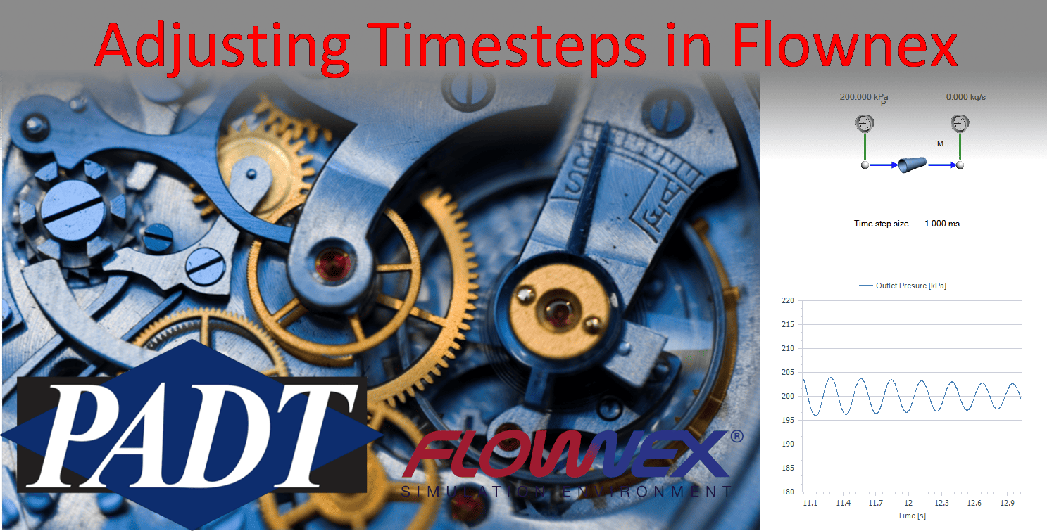
The simulation runs faster until the moment before mass flow is reduced. We are than able to capture pressure oscillations with a higher resolution by ramping our timestep down.
Closing Thoughts
Now we have learned a bit more about how the adaptive timestep operates and how we can modify the timestep property during a simulation. Timesteps may be adjusted in Flownex to reduce simulation time, or to ensure that reasonable truncation errors are achieved in a simulation. These tools are helpful for efficiently running transient simulations with multiple timescales.


