
Introduction
When doing electromagnetic simulations, we often want to know what current is flowing through an object other than the one we are exciting – eddy currents. There’s a lot going on within Maxwell’s equations related to this topic, but we’re going to focus on one simple equation:
∮H∙dl=I_enc
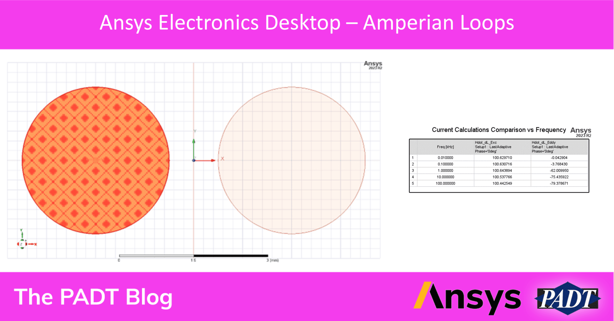
Which is the integral form of Ampere’s Circuital Law, and we’ll show how you can use the field calculator to find that enclosed current using the fields that Maxwell calculates for you! For this example, we are going to be using a simple case of two adjacent copper wires – the one on the left is excited with a 100 Amp current coming out of the screen (+Z), and the other is not excited at all.

Measurement Setup
The first step is to make a closed loop around the object of interest – we’ll be doing this by drawing a 2D circle that fully surrounds our non-excited wire. There isn’t an exact diameter value, we just need to make sure the circle fully surrounds a cross section of just the wire.

And now we have a circle, and we need to convert it to a closed loop that doesn’t have a covered face. To do this, we select our circle, right click, and navigate to Extend Selection -> All Object Edges. This will select just the edge of our circle, which we will then turn into a unique object using either Modeler -> Edge -> Create Object from Edge in the menus on the top bar, or select it from the Draw ribbon:

The circle can be deleted now, we just wanted the edges (kind of like when eating homemade brownies). The edge will have a ridiculously long name – by default something like “Circle1_ObjectFromEdge1.” Feel free to rename it to anything you desire, just remember what it is when going through the field calculator. In this example, it was named “Current_Sense_Eddy.”
Field Calculator
or, How I Learned to Love Reverse Polish Notation
The easiest way to open the fields calculator is to right click on “Field Overlays” in the project manager and select the “Calculator” option. This will open the fields calculator, which we will use to generate our expressions for current.

Below is a table showing the calculator operations, and what the stack will look like after each step – handy for following along.
| Calculator Operation | Resulting Stack Display (top entry only unless noted) |
| Input: Quantity -> H | CVc : <Hx,Hy,0> |
| General: Smooth | CVc : Smooth(<Hx,Hy,0>) |
| Input: Function -> Scalar -> Phase | Scl : Phase CVc : Smooth(<Hx,Hy,0>) |
| General: Complex -> AtPhase | Vec : AtPhase(Smooth(<Hx,Hy,0>), Phase) |
| Vector: Unit Vec -> Tangent | Vec : LineTangent |
| Vector: Dot | Scl : Dot(AtPhase(Smooth(<Hx,Hy,0>), Phase), LineTangent) |
| Input: Geometry -> Line -> Current_Sense_Eddy | Lin : Line(Current_Sense_Eddy) |
| Scalar: ∫ (Integrate) | Scl : Integrate(Line(Current_Sense_Eddy), Dot(AtPhase(Smooth(<Hx,Hy,0>), Phase), LineTangent)) |
And then we have our final expression – that whole mess of words represents the same equation as we showed before, where the contour that is being integrated over is the edge of the circle we drew! We can save this value as a Named Expression, and then use it in future reports – we’ll call ours Hdot_dL_Eddy.

The same process can be used to create a measurement loop around the excited wire (with a new circle) so we can verify we’re getting the right current. We’ll name that expression Hdot_dL_Exc, so now we have an expression for the Amperian loop current in both our excited wire and the one that we want to extract eddy currents from. We’ll create a data table of our two calculated currents and see how they change with frequency.
Results

Our excited wire is measuring around 100 Amps – a positive sign since that is what we set it to be! The other wire’s current increases with frequency and is negative, both of which make sense from Maxwell’s equations – another positive sign. Our Amperian loop is accurately measuring the current in our two wires! This method can be done with any closed loop, in both 2D and 3D solvers, if it is a line object that completely encapsulates a cross-sectional area where current is flowing.
A Few Final Words
Now we all have a handy method of measuring current in eddy current solutions, and all we needed was a couple circles and a little bit of Reverse Polish Notation from our fields calculator!


