PyAnsys Tutorial – Exporting Ansys Results in 3D File Formats, Part 2

A few months ago, I decided it was time for me to buckle down and learn PyAnsys. We also needed a replacement for our Ansys ACT tool that output results in a 3MF file format, which became out of date. This series is the result of that effort, sharing with you all that I learned along the way.

In Part 1 of this series, we covered:

1. How to install and set up PyAnsys on your machine
2. Create a PyAnsys script that reads an Ansys Mechanical result file
3. Pull mesh and results from the file
4. Plot results to the screen using Python
5. Write a VTK file of the results
   

If you have not run PyAnsys before, then please go back to the first post and make sure you add the PyAnsys modules to your Python install using pip as shown. Some users have had issues with out of date modules when they tried to use this software.

Just to whet your appetite, here are some of the things we have plotted on our Stratasys J55 and J850 Polyjet printers:

Let’s Use PyAnsys to Write a File That We Can Use to 3D Print Results

Creating a VTK file lets you use other tools to convert to other formats, but when push comes to shove, we want to write 3D files directly and skip the extra step. We also need to do more than create files with equivalent stress from the first solution set in the file.

That is why, in Part 2, we are going to:

1. Parameterize things
2. Support multiple result types
3. Distort the mesh
4. Write a WRL/VRML file we can use for 3D Printing

We will step through each bit of code for each of these steps. The zip file at the bottom of this post will have it all in one file, but you can also copy and paste as we go.

1: Clean Things Up and Add Parameters

In this first section of the code, we will do pretty much the same thing we did in that section for Part 1 of these tutorials. The big difference is some new modules and more parameters to support new capabilities. As you can see we will use pyvista and numpy. You will see why later on.

Then we create new parameters for other result types, how much distortion scaling we want, and support for more than one output format. Nothing fancy here.

#### SECTION 1 ####

#1.1: Get all modules loaded
from ansys.dpf import post
from ansys.dpf import core as dpf
from ansys.dpf.core import operators as coreops
from ansys.dpf.core import fields_container_factory
from ansys.dpf.core.plotter import DpfPlotter

# For the new capabilities, we need pyvista, and numpy along with os
import pyvista as pv
import numpy as np
import os

# 1.2: Specify variables for filenames and directory
#      Make sure you change this to your directory and RST file
#      Note that Python converst / to \ on windows so you don't have to. 
rstFile = "twrtest1-str.rst"
rstDir = "C:/Users/eric.miller/OneDrive - PADT/Development/pyAnsys/twrtest/"
outroot= "twrtest1"

#1.3: Now define some parameters we will need to 
#     get other result types, scale distortion, and write to more than one format

# They ansys value to retrieve. Valid result types are: 
#     ux, uy,uz, usum, seqv, s1,s2,s3,sx,sy,sz, sxy, sxz, syz, tmp
rsttype = "usum"

# A scale factor for the max deflection value on the 
# model as a percent of the largest value of the bounding box
pcntdfl = 5

# The 3d result file format. For now we will check for vtk or wrl
outtype = "wrl"

# The result step/mode to grab
rstnum = 1

#1.4: Build the output file name from the file root and 
#     the result type and file type
outfname = outroot + "-" + rsttype + "-" + str(rstnum) + "." + outtype

#1.5: Let the user know what you have
print ("==========================================================================")
print ("Starting the translation of your Ansys results to a different file format")
print ("  Input file: ", rstFile)
print ("  Directory: ", rstDir)
print ("  Output file: ", outfname)
print ("  Solution step/mode: ", rstnum)
print ("  Result type: ", rsttype)
print ("  Percent deflection distortion: ", pcntdfl)
print ("-------------------------------------------------------------------------")

2: Open the file, get mesh, and get the right stress value

As mentioned in Part 1, opening the file and getting the mesh is so easy, you almost feel like you left something out. Things get more complicated with a bunch of if statements looking for the type of result to read. You can see that there is a displacement, stress, and thermal object and each has a slightly different way of grabbing value. This section could use some error checking if you want to add it.

Note how when we grab the temperature, displacement, and stress values, we are now specifying a result number. It is not by load-step, sub-step. Whatever you want, put it into rstval to use in making the plot and the file.

If this section looks confusing, go back and review section 2 from the first part of this tutorial.

#### SECTION 2 ####

#2.1: Open the result file and load the solution and mesh
os.chdir(rstDir)
path = os.getcwd()
mysol = post.load_solution(rstFile)
mymesh = mysol.mesh

#2.2: Grab the results from the specified solution step, 
#     then get the request result type (thermal or displacement and stress)
print ("++ Getting result information from file")

# Displacement, stress, and thermal for the solution set number
if rsttype == "tmp":
    thrm1 = mysol.temperature(set=rstnum)
else:
    dsp1 = mysol.displacement(set=rstnum)
    str1 = mysol.stress(set=rstnum)

#2.3: Use an if statement to pull in the specific result values

# Start with displacement
if rsttype == "u":
    rstval = dsp1.vector.result_fields_container
elif rsttype == "ux":
    rstval = dsp1.x.result_fields_container
elif rsttype == "uy":
    rstval = dsp1.y.result_fields_container
elif rsttype == "uz":
    rstval = dsp1.z.result_fields_container
elif rsttype == "usum":
    rstval = dsp1.norm.result_fields_container

# Now check for stresses
elif rsttype == "seqv":
    rstval = str1.von_mises.result_fields_container
elif rsttype == "s1":
    rstval = str1.principal_1.result_fields_container
elif rsttype == "s2":
    rstval = str1.principal_2.result_fields_container
elif rsttype == "s3":
    rstval = str1.principal_3.result_fields_container
elif rsttype == "sx":
    rstval = str1.xx.result_fields_container
elif rsttype == "sy":
    rstval = str1.yy.result_fields_container
elif rsttype == "sz":
    rstval = str1.zz.result_fields_container
elif rsttype == "sxy":
    rstval = str1.xy.result_fields_container
elif rsttype == "sxz":
    rstval = str1.xz.result_fields_container
elif rsttype == "syz":
    rstval = str1.yz.result_fields_container

# Last, do temperatures
elif rsttype == "tmp":
    rstval = thrm1.scalar.result_fields_container

3. Grab deflections and distort the mesh

Here is our first completely new section. Since we want to show results on a distorted mesh, we have to get the displacement values, multiply them by a scale factor, then move the nodes to their deflected locations. As with everything in Python, there are dozens of methods and functions to help with this. For this code, I kept things kind of simple.

First we figure out how big the model is, then get the max displacement for the result set we are working with. Knowing that value, we can now calculate a scale factor using the user’s input. We use the math operators in PyAnsys to first scale the deflection values, then to add those values to the nodal position.

#### SECTION 3 #####

# 3.1: If this is thermal, just copy the 
#      undistored mesh to the variables we will us to plot and write 
if rsttype == "tmp": 
    dflmesh = mymesh.deep_copy()
    newcoord = dflmesh.nodes.coordinates_field
else:
    #3.2: Not thermal so get info needed to calculate a distorted mesh
    print("++ Calculating deflection distortion")

    # Grab the total distortion at each node
    usumval = dsp1.vector.result_fields_container

    # Get model extents. Feed the min_max operator "mymesh"
    extop = dpf.operators.min_max.min_max(mymesh.nodes.coordinates_field)
    coordmin = extop.outputs.field_min()
    coordmax = extop.outputs.field_max()
    
    # Look at the X, Y, Z min and max coordinate 
    #   value and find the biggest demention of the mesh
    #   There is probably a clever python way to do this in one line
    dltmax =0.0
    for i in range(0,3):
        if (coordmax.data[i]-coordmin.data[i]) > dltmax:
            dltmax = coordmax.data[i]-coordmin.data[i]

    # Get the maximum deflection value from usumval
    umaxop = dpf.operators.min_max.min_max(field=usumval)
    umax = 0.0
    for i in range(0,3):
        if umaxop.outputs.field_max().data[i] > umax:
                umax = umaxop.outputs.field_max().data[i]

    # Calculate a scale factor that is the specified 
    #   percentage of the max deflection devided by the max size
    dflsf = pcntdfl/100.0
    sclfact = dflsf*dltmax/umax

    #3.3: Scale the deflection values then distort the nodal coordinates 
    
    # Get a copy of the mesh to distort
    dflmesh = mymesh.deep_copy()
    newcoord = dflmesh.nodes.coordinates_field

    # Scale the deflection field by the scale factor
    sclop = dpf.operators.math.scale(usumval,float(sclfact))
    scaledusum = sclop.outputs.field()

    # Add the scaled deflection field to the nodal positions
    addop = dpf.operators.math.add(newcoord, scaledusum)
    tempcoord = addop.outputs.field()

    # Overwrite the nodal positions of dflmesh with the deflected ones
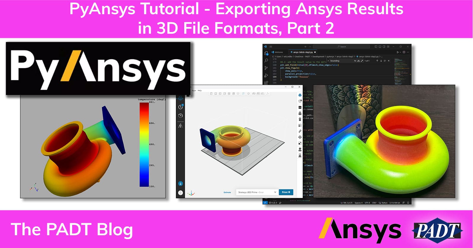
    newcoord.data = tempcoord.data

4. Create a plot to the screen to verify what you have

No changes here from before, just build a simple window and show it. To exit the window, close it or press q.

#### SECTION 4 ####
#4.1: create a Pyansys plotter object first
print ("++ Making plot (press q to exit)")
plt = DpfPlotter()

#4.2: add the result value to the deflected mesh and the plot
plt.add_field(rstval[0],dflmesh,show_edges=False)
plt.show_figure(
    show_axes=True,
    parallel_projection=False,
    background="#aaaaaa",
)

Here is what I end up with for a thermal model I use (rth included in zip file)

5: Write out a VTK or WRL File

Here is where we get a bit fancy. First we use an if/elif to use the write code for either VTK or WRL.

For that WRL file, PyAnsys doesn’t have a tool to write to WRL, so we have to use pyvista. And Pyvista can’t take the PyAnsys results directly. We have to move the nodal or elemental result info from the result objects into what pyvista calls a grid as either point data or cell data. Once we do that, we can feed that grid to the pyvista plotter tools, and use export_vrml to write the file.

#### SECTION 5 ####

#5.1: I writing a VTK file, then do the same thing we did for the first post
#      setup a pyansys vtk_export operator, add mesh, filename, 
#      and result values, then run teh operator
print ("++ Making output file")
if outtype == "vtk":
    vtkop = coreops.serialization.vtk_export() 
    vtkop.inputs.mesh.connect(dflmesh)

    vtkop.inputs.file_path.connect(outfname)
    vtkop.inputs.fields1.connect(rstval)

    vv = vtkop.run()
    print(vv)
    print ("++ Results written to: " + outfname)

#5.2: If doing a WRL, use pyVista to create a VRML file for visualization 
#     and 3D Printing
#     The pyvista module does not work with the Ansys mesh object, 
#     so you have to do some fancy converstion to get the mesh into a 
#     grid it can use
#     It also doesn't automatically handle element values vs nodal value, 
#     so we have to handle that
elif outtype == "wrl":
    # Get the result field and the deflected mesh into some variables. 
    field = rstval[0]
    meshed_region = dflmesh

    # We are going to need the name of the field in "field" 
    # in order to grab it later
    fieldName = '_'.join(field.name.split("_")[:-1])

    # Look in the field to see if the location of the results is nodal or elemental
    if field.location == dpf.locations.nodal:
        mesh_location = meshed_region.nodes
    elif field.location == dpf.locations.elemental:
        mesh_location = meshed_region.elements
    else:
        raise ValueError(
            "Only elemental or nodal location are supported for plotting."
        )

    # Next we are going to use a mask to get a grid them assign resutls to 
    # either the element or nodal data
    overall_data = np.full(len(mesh_location), np.nan) 
    ind, mask = mesh_location.map_scoping(field.scoping)
    overall_data[ind] = field.data[mask]
    grid = meshed_region.grid
    if field.location == dpf.locations.nodal:
        grid.point_data[fieldName] = overall_data
    elif field.location == dpf.locations.elemental:
        grid.cell_data[fieldName] = overall_data

#5.3: Now that we have a grid and values on the grid, 
#     use the pyvista plotter operator to make the file
    objplt = pv.Plotter()
    objplt.add_mesh(grid) #close, data is not lined up with nodes
    objplt.export_vrml(outfname)
    print ("++ Results written to: " + outfname)

#5.4: Close out
print ("---------------------------------------------------------------------------")
print ("Done")

And, here is what it looks like in Stratasys GrabCad, ready to go into our J850 Prime system.

And what it looks like in the real world:

Next Steps for Our PyAnsys Journey

You can find the Python script, result files for my test model and the housing shown above, and some WRL files I made in this zip file:

As you can see, the code as is works if you need VTK or WRL, and you just need to use it occasionally. To make things more useful, in the next part of this series, we will add a graphical user interface (GUI) and support a few more file formats.

When you are ready, you can move on to Part 3.

If this stuff gets you interested in doing more automation with PyAnsys scripting, but you don’t have the time to do it yourself, contact PADT at consult@padtinc.com, and we can talk about how we can help.